2 Sampling Distribution

statistical inference

sampling distribution

Author

Rodolfo Lourenzutti

Learning objectives

Define the sampling distribution of a statistic, and explain why it is the central concept of statistical inference.
Distinguish between the population distribution, the sample distribution, and the sampling distribution, three conceptually distinct objects that are easy to confuse.
Use simulation to approximate and explore a sampling distribution, and describe its two key properties: center (bias/unbiasedness) and spread (standard error).
Distinguish between a statistic as a random variable (the estimator) and the specific value it takes in a given sample (the estimate), and explain why this distinction matters.
Explain how sample size affects the precision of an estimate, and describe the law of diminishing returns in sampling.
Use rep_sample_n() from the infer package to simulate a sampling distribution, and use summarise() to compute the statistic of interest for each sample.

Introduction

In the previous chapter, we learned how to take a random sample and compute a statistic (such as the sample mean) to estimate a population parameter. We pick up with the same shipment of $50{,}000$ Apple screens (screens_pop) and the sample of $300$ screens (screens_sample) from before. We also saw that because samples are random, everything about the sample is random, including the statistic we compute from it. We call this sampling variability. Take a look at the code below and notice how two random samples yield different sample proportions.

Since we are using statistics (which are random) to estimate parameters (which are fixed), one could argue that any value we get from a single sample is just a lucky (or unlucky) draw that does not necessarily reflect the true population parameter.

Let’s think this through together! Suppose the true proportion of screens that can withstand a crack pressure of $750$ psi or more is $p = 0.95$. Since we cannot test all $50{,}000$ screens, we have to rely on our single sample. But here is the catch: we already know that a different random sample would have given a different sample proportion. So, how can we possibly trust the one estimate we happen to have?

Imagine a scenario where every possible sample yields a sample proportion, $\hat{p}$, very close to $p = 0.95$. In that world, we could relax knowing our single estimate is definitely close to the truth. In this scenario, there is still sampling variability, but since all samples give sample proportions that are very close to the true proportion, the fluctuation is irrelevant.

On the other hand, if different samples produced wildly different proportions (jumping around, say, from $0.7$ to $0.8$ or $0.99$), our single estimate could be miles away from the truth, and we would have no way of knowing it. In this scenario, the sampling variability is huge, and our single estimate is not reliable at all.

In practice, we are rarely in either of these extreme worlds. We are usually somewhere in between, where some samples yield poor estimates (i.e., far from the true parameter), while other samples yield good estimates (i.e., close to the true parameter). Luckily, most samples give estimates that are reasonably close to the true parameter, and the samples that yield terrible estimates are relatively rare. But how rare? Since we cannot evaluate how good a given estimate is on its own, we need to be able to quantify how likely it is that we get a good estimate versus a bad one.

To properly study this variability, we need to look at the distribution of the statistic (in this case the sample proportion) across all possible samples. This is called the sampling distribution and it is the central concept of statistical inference.

Definition 2.1 (Sampling Distribution) The sampling distribution of a statistic is the distribution of that statistic computed from all possible samples of a given size $n$ drawn from the population.

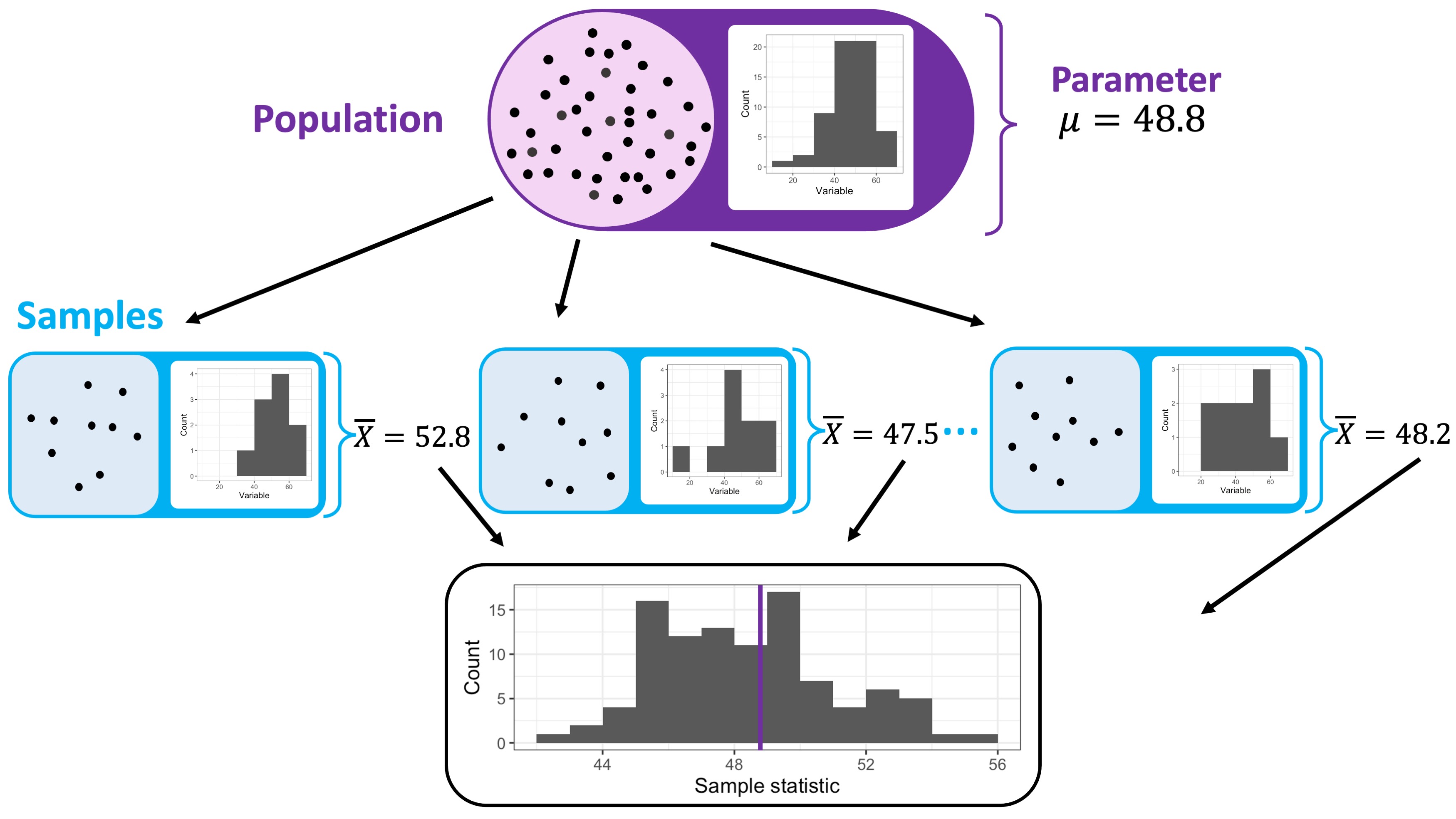
Figure 2.1 puts the whole picture together: the population has a fixed (but unknown) parameter; each sample we could draw yields its own statistic; and the sampling distribution is what we get by collecting the statistic from every possible sample. Notice that it is a distribution of statistics ($\bar{X}$ values), not of the variable of interest (a distinction that trips students up constantly, so keep it in mind as we go forward).

Figure 2.1: From population to sampling distribution: every possible sample yields its own statistic $\bar{X}$; collecting these statistics across all possible samples builds the sampling distribution shown at the bottom (purple line marks the population parameter $\mu$).

2.1 The Sampling Distribution, Exactly

Let’s start with a small population and a small sample size, so that we can enumerate every possible sample and compute the statistic for each one. This will allow us to see the sampling distribution exactly.

Example 2.1 An aquarium has $20$ fish. You are responsible for feeding them, and to determine the right amount of food, you need to know their average weight. You decide to estimate the population mean by sampling $3$ fish at random. The weights of all 20 fish in the population are shown in Table 2.1 (measured in decagrams, dkg).

Table 2.1: The weights of the 20 fish in the aquarium. (Note: 1 dkg = 10 g).
(Population mean μ = 43.45 dkg)

Fish	Weight (dkg)	Fish	Weight (dkg)	Fish	Weight (dkg)	Fish	Weight (dkg)
Fish #1	43	Fish #6	44	Fish #11	26	Fish #16	42
Fish #2	46	Fish #7	41	Fish #12	47	Fish #17	36
Fish #3	47	Fish #8	40	Fish #13	37	Fish #18	36
Fish #4	59	Fish #9	43	Fish #14	42	Fish #19	61
Fish #5	24	Fish #10	58	Fish #15	60	Fish #20	37

With only $20$ fish and a sample size of $n = 3$, there are exactly $\binom{20}{3} = 1{,}140$ possible samples we could get. The table below lists all $1{,}140$ possible samples as well as their sample means. Below the table, Figure 2.2 shows the histogram of the sampling distribution (you can click a bar in the histogram to highlight the corresponding samples in the table that yield a sample mean in that bin).

Table 2.2: All 1,140 possible samples sorted by fish numbers.
(Click one or more bars in the histogram below to highlight samples.)

fish_wt = [43, 46, 47, 59, 24, 44, 41, 40, 43, 58,
           26, 47, 37, 42, 60, 42, 36, 36, 61, 37]

fish_pop_mean_ojs = 43.45

// ── Generate all C(20,3) = 1140 samples ───────────────────────────────────────
all_fish_samples = {
  const rows = [];
  for (let i = 0; i < 20; i++) {
    for (let j = i + 1; j < 20; j++) {
      for (let k = j + 1; k < 20; k++) {
        const w = [fish_wt[i], fish_wt[j], fish_wt[k]];
        const m = +(w[0] + w[1] + w[2]).toFixed(2) / 3;
        rows.push({
          "Sample"            : `(#${i+1}, #${j+1}, #${k+1})`,
          "Sample mean (dkg)" : +m.toFixed(2)
        });
      }
    }
  }
  return rows;
}

// ── Mutable state ─────────────────────────────────────────────────────────────
mutable fish_sel      = []     // Array of selected bins: [{x0, x1}, ...]
mutable fish_rows_shown = 12

// ── All-samples table (3 per row, highlight on click) ─────────────────────────
{
  // Sort all 1140 samples by fish numbers (natural generation order)
  const sorted = all_fish_samples.slice();

  const sel       = fish_sel;
  const COLS      = 3;          // samples per table row
  const STEP      = 12;         // rows to add per click
  const totalRows = Math.ceil(sorted.length / COLS);   // 380 rows
  const shownRows = Math.min(fish_rows_shown, totalRows);

  // ── Style block ──────────────────────────────────────────────────────────────
  const styleBlock = html`<style>
    .ojs-samples-table {
      font-size: 13.5px !important;
      margin-top: 8px !important;
      margin-bottom: 8px !important;
      border-collapse: collapse !important;
      border: none !important;
      font-family: var(--bs-body-font-family, "Inter", -apple-system, sans-serif) !important;
    }
    
    /* Header cells styling to match Table 1 */
    .ojs-samples-table thead th {
      background-color: #2c3e50 !important;
      color: #ffffff !important;
      font-weight: 600 !important;
      font-size: 14.5px !important;
      padding: 0.8rem 1rem !important;
      border: none !important;
      white-space: nowrap !important;
      vertical-align: middle !important;
      text-align: left !important;
    }
    
    /* Center align the Mean Weight header */
    .ojs-samples-table thead th.num-col {
      text-align: center !important;
    }
    
    /* Separator header cell styling to make a solid continuous banner */
    .ojs-samples-table thead th.table-sep {
      background-color: #2c3e50 !important;
      padding: 0 !important;
      width: 16px !important;
      max-width: 16px !important;
      min-width: 16px !important;
      border: none !important;
    }

    /* Body cell styling to match Table 1 */
    .ojs-samples-table tbody td {
      padding: 0.8rem 1rem !important;
      vertical-align: middle !important;
      text-align: left !important;
      border-bottom: 1px solid rgba(0, 0, 0, 0.05) !important;
      font-size: 14px !important;
    }

    /* Center-align numeric columns in body */
    .ojs-samples-table tbody td.num-col {
      text-align: center !important;
    }

    /* Zebra striping (even rows) to match Table 1 */
    .ojs-samples-table tbody tr:nth-child(even) td:not(.lit-cell) {
      background-color: rgba(0, 0, 0, 0.015) !important;
    }
    
    /* Hover styling to match Table 1 */
    .ojs-samples-table tbody tr:hover td:not(.lit-cell) {
      background-color: rgba(0, 0, 0, 0.035) !important;
      transition: background-color 0.2s ease;
    }

    /* Highlighted cells on click */
    .ojs-samples-table td.lit-cell {
      background-color: rgba(255, 99, 71, 0.12) !important;
      color: tomato !important;
      font-weight: bold;
    }

    /* Separator body cell styling */
    .ojs-samples-table tbody td.table-sep {
      background-color: transparent !important;
      background: transparent !important;
      border: none !important;
      padding: 0 !important;
      width: 16px !important;
      max-width: 16px !important;
      min-width: 16px !important;
    }
  </style>`;

  // ── Status message ───────────────────────────────────────────────────────────
  let statusEl;
  if (sel && sel.length > 0) {
    const count = sorted.filter(
      d => sel.some(item => d["Sample mean (dkg)"] >= item.x0 && d["Sample mean (dkg)"] < item.x1)
    ).length;
    statusEl = html`<p style="color:tomato; font-weight:bold; margin:10px 0 6px;">
      ${count} sample${count !== 1 ? "s" : ""} highlighted in the selected mean intervals.
      Click a highlighted bar again to deselect, or click Reset in the histogram to clear all.
    </p>`;
  } else {
    statusEl = html`<p style="color:#555; margin:0 0 6px;">
      
    </p>`;
  }

  // ── Table header row ─────────────────────────────────────────────────────────
  const headerCells = [];
  for (let c = 0; c < COLS; c++) {
    if (c > 0) headerCells.push(html`<th class="table-sep"></th>`);
    headerCells.push(html`<th>Sampled Fish</th>`);
    headerCells.push(html`<th class="num-col">Mean Weight<br>(dkg)</th>`);
  }
  const headerRow = html`<tr>${headerCells}</tr>`;

  // ── Data rows ────────────────────────────────────────────────────────────────
  const dataRows = [];
  for (let r = 0; r < shownRows; r++) {
    const cells = [];
    for (let c = 0; c < COLS; c++) {
      const idx = r * COLS + c;
      if (c > 0) cells.push(html`<td class="table-sep"></td>`);
      if (idx < sorted.length) {
        const row  = sorted[idx];
        const mean = row["Sample mean (dkg)"];
        const lit  = sel && sel.length > 0 && sel.some(item => mean >= item.x0 && mean < item.x1);
        const cellClass = lit ? "lit-cell" : "";
        const meanClass = lit ? "lit-cell num-col" : "num-col";
        cells.push(html`<td class="${cellClass}">${row["Sample"]}</td>`);
        cells.push(html`<td class="${meanClass}">${mean}</td>`);
      } else {
        cells.push(html`<td></td>`);
        cells.push(html`<td></td>`);
      }
    }
    dataRows.push(html`<tr>${cells}</tr>`);
  }

  // ── Buttons ──────────────────────────────────────────────────────────────────
  const remaining = totalRows - shownRows;
  const btnStyle  = "padding:4px 12px; font-size:13px; cursor:pointer; margin-right:6px;";
  const btnContainer = html`<div style="margin-top:8px;">`;

  if (shownRows < totalRows) {
    const nextBatch  = Math.min(STEP, remaining);
    const showMoreBtn = html`<button style="${btnStyle}">Show ${nextBatch} more rows (${remaining} remaining)</button>`;
    showMoreBtn.addEventListener("click", () => { mutable fish_rows_shown = shownRows + STEP; });
    btnContainer.append(showMoreBtn);

    if (shownRows + STEP < totalRows) {
      const showAllBtn = html`<button style="${btnStyle}">Show all ${totalRows} rows</button>`;
      showAllBtn.addEventListener("click", () => { mutable fish_rows_shown = totalRows; });
      btnContainer.append(showAllBtn);
    }
  }

  if (shownRows > STEP) {
    const collapseBtn = html`<button style="${btnStyle}">↑ Collapse</button>`;
    collapseBtn.addEventListener("click", () => {
      mutable fish_rows_shown = STEP;
      setTimeout(() => {
        const el = document.getElementById("tbl-fish-sampling-dist");
        if (el) {
          el.scrollIntoView({ behavior: "smooth", block: "start" });
        }
      }, 50);
    });
    btnContainer.append(collapseBtn);
  }

  // ── Assemble ─────────────────────────────────────────────────────────────────
  const wrapper = html`<div></div>`;
  wrapper.append(styleBlock);
  const table = html`<table class="table ojs-samples-table">
    <thead>${headerRow}</thead>
    <tbody>${dataRows}</tbody>
  </table>`;
  wrapper.append(table);
  if (btnContainer.children.length > 0) wrapper.append(btnContainer);
  wrapper.append(statusEl);
  return wrapper;
}

viewof show_true_mean = {
  const form = html`<form style="display: inline-flex; align-items: center; margin: 0; padding: 0;">
    <label style="display: inline-flex; align-items: center; gap: 8px; margin: 0; padding: 0; cursor: pointer; user-select: none; font-size: 14.5px; font-weight: 500; color: var(--bs-body-color); line-height: 1;">
      <input type="checkbox" style="cursor: pointer; width: 16px; height: 16px; margin: 0 !important; padding: 0 !important; accent-color: #0284c7; flex-shrink: 0;">
      <span style="display: inline-block; line-height: 1;">Show population mean <span style="color:tomato; font-weight: bold;">(μ = 43.45)</span></span>
    </label>
  </form>`;
  
  const input = form.querySelector("input");
  input.addEventListener("change", () => {
    form.value = input.checked;
    form.dispatchEvent(new CustomEvent("input"));
  });
  
  form.value = false;
  return form;
}

// ── Interactive histogram ──────────────────────────────────────────────────────
{
  const sel      = fish_sel || [];
  const showMean = show_true_mean;

  const W = 640, H = 480;
  const margin = { top: 65, right: 20, bottom: 65, left: 65 };

  // Bin all 1140 sample means with a set domain to ensure equal width bins
  const thresholds = d3.range(29, 62, 2.5);
  const binner = d3.bin()
    .value(d => d["Sample mean (dkg)"])
    .domain([26, 62])
    .thresholds(thresholds);
  const bins = binner(all_fish_samples);

  const x = d3.scaleLinear()
    .domain([bins[0].x0 - 0.3, bins[bins.length - 1].x1 + 0.3])
    .range([margin.left, W - margin.right]);

  const y = d3.scaleLinear()
    .domain([0, d3.max(bins, d => d.length) + 10])
    .range([H - margin.bottom, margin.top]);

  // Create relative outer container to position the Reset Selection button inside the plot cell
  const container = html`<div style="position: relative; width: ${W}px; margin: 0 auto;"></div>`;

  const svg = d3.create("svg")
    .attr("width", W).attr("height", H)
    .style("font-family", "sans-serif").style("font-size", "13px");

  // Create premium reset button absolute positioned at the top-right
  const resetBtn = html`<button style="
    position: absolute;
    top: ${margin.top}px;
    right: ${margin.right}px;
    z-index: 10;
    padding: 6px 14px;
    font-size: 12.5px;
    font-weight: 600;
    cursor: pointer;
    border: none;
    border-radius: 6px;
    background: #0284c7; /* Vibrant modern blue */
    color: #ffffff;
    transition: background 0.15s, transform 0.15s, box-shadow 0.15s;
    box-shadow: 0 4px 12px rgba(2, 132, 199, 0.25);
  ">↺ Reset Selection</button>`;

  resetBtn.addEventListener("mouseover", () => {
    resetBtn.style.background = "#0369a1"; // Elegant deep ocean blue
    resetBtn.style.boxShadow = "0 6px 16px rgba(2, 132, 199, 0.35)";
    resetBtn.style.transform = "translateY(-1px)";
  });
  resetBtn.addEventListener("mouseout", () => {
    resetBtn.style.background = "#0284c7";
    resetBtn.style.boxShadow = "0 4px 12px rgba(2, 132, 199, 0.25)";
    resetBtn.style.transform = "translateY(0)";
  });
  resetBtn.addEventListener("click", () => {
    mutable fish_sel = [];
  });

  if (sel.length > 0) {
    container.append(resetBtn);
  }

  // Plot Title
  svg.append("text")
    .attr("x", W / 2).attr("y", margin.top - 36)
    .attr("text-anchor", "middle")
    .attr("fill", "var(--bs-body-color, #111)")
    .attr("font-size", "17px").attr("font-weight", "600")
    .style("font-family", "system-ui, -apple-system, sans-serif")
    .text("Sampling Distribution of the Sample Mean");

  // Instruction subtitle
  svg.append("text")
    .attr("x", W / 2).attr("y", margin.top - 12)
    .attr("text-anchor", "middle")
    .attr("fill", "#666").attr("font-size", "12px")
    .text("Click one or more bars to highlight samples in the table above · click again to deselect");

  // Helper: check if a bin is selected
  const isBinSelected = d => sel.some(item => item.x0.toFixed(3) === d.x0.toFixed(3));

  // Bars
  const bars = svg.append("g").selectAll("rect").data(bins).join("rect")
    .attr("x",      d => x(d.x0) + 1)
    .attr("width",  d => Math.max(0, x(d.x1) - x(d.x0) - 1))
    .attr("y",      d => y(d.length))
    .attr("height", d => y(0) - y(d.length))
    .attr("fill",   d => isBinSelected(d) ? "tomato" : "steelblue")
    .style("cursor", "pointer");

  // Count label on selected bars
  if (sel.length > 0) {
    sel.forEach(item => {
      const selBin = bins.find(d => d.x0.toFixed(3) === item.x0.toFixed(3));
      if (selBin) {
        svg.append("text")
          .attr("x", (x(selBin.x0) + x(selBin.x1)) / 2)
          .attr("y", y(selBin.length) - 5)
          .attr("text-anchor", "middle")
          .attr("font-size", "11px").attr("fill", "tomato").attr("font-weight", "bold")
          .text(selBin.length);
      }
    });
  }

  // Hover: lighten bar and show count
  bars.on("mouseover", function(event, d) {
    const isSelected = isBinSelected(d);
    if (!isSelected) d3.select(this).attr("fill", "#4a8ab5");
    if (!isSelected) {
      svg.append("text").attr("class", "hover-count")
        .attr("x", (x(d.x0) + x(d.x1)) / 2)
        .attr("y", y(d.length) - 5)
        .attr("text-anchor", "middle")
        .attr("font-size", "11px").attr("fill", "#333")
        .text(d.length);
    }
  }).on("mouseout", function(event, d) {
    const isSelected = isBinSelected(d);
    if (!isSelected) d3.select(this).attr("fill", "steelblue");
    svg.selectAll(".hover-count").remove();
  });

  // Click: toggle selection (support multi-select)
  bars.on("click", function(event, d) {
    const index = sel.findIndex(item => item.x0.toFixed(3) === d.x0.toFixed(3));
    if (index > -1) {
      // Remove from selection
      mutable fish_sel = sel.filter((_, i) => i !== index);
    } else {
      // Add to selection
      mutable fish_sel = [...sel, { x0: d.x0, x1: d.x1 }];
    }
  });

  // Population mean line (toggled)
  if (showMean) {
    svg.append("line")
      .attr("x1", x(fish_pop_mean_ojs)).attr("x2", x(fish_pop_mean_ojs))
      .attr("y1", margin.top).attr("y2", H - margin.bottom)
      .attr("stroke", "red").attr("stroke-width", 2)
      .attr("stroke-dasharray", "6 3");
    svg.append("text")
      .attr("x", x(fish_pop_mean_ojs) + 6).attr("y", margin.top + 18)
      .attr("fill", "red").attr("font-size", "12px")
      .text(`μ = ${fish_pop_mean_ojs}`);
  }

  // X axis
  svg.append("g")
    .attr("transform", `translate(0,${H - margin.bottom})`)
    .call(d3.axisBottom(x).ticks(10));
  svg.append("text")
    .attr("x", W / 2).attr("y", H - 10)
    .attr("text-anchor", "middle").attr("font-size", "14px")
    .text("Sample Mean Weight (dkg)");

  // Y axis
  svg.append("g")
    .attr("transform", `translate(${margin.left},0)`)
    .call(d3.axisLeft(y).ticks(6));
  svg.append("text")
    .attr("transform", "rotate(-90)")
    .attr("x", -(H / 2)).attr("y", 16)
    .attr("text-anchor", "middle").attr("font-size", "14px")
    .text("Count (number of samples)");

  container.append(svg.node());
  return container;
}

Figure 2.2: Sampling distribution of the sample mean weight across all 1,140 possible samples of 3 fish. Click a bar to highlight the corresponding samples in the table above. Click again to deselect.

□

Exercise 2.1 Using the interactive histogram above, answer the following questions.

(a) What is the smallest sample mean you can find? How many samples give this minimum sample mean? Which fish are in these samples?

Smallest sample mean: 28.67 dkg (approximately 286.7 grams).
Number of samples: 2 samples that yield this minimum mean.
- Sample 1: (Fish #5, Fish #11, Fish #17) (weights: 24, 26, and 36 dkg)
- Sample 2: (Fish #5, Fish #11, Fish #18) (weights: 24, 26, and 36 dkg)

The leftmost bar in the histogram corresponds to these two samples, which are among the unluckiest possible samples, giving the worst underestimates of the true population mean ($\mu = 43.45$ dkg).

(b) Click on bars to select all samples whose mean falls between $40$ and $46$ dkg. How many such samples are there?

viewof answer_fish_1a = Inputs.radio(
  ["Less than 300",
   "Between 300 and 500",
   "Between 500 and 700",
   "More than 700"],
  {label: "Number of samples: "}
)

viewof answer_fish_1c = Inputs.radio(
  ["29 to 39 dkg",
   "39 to 49 dkg",
   "49 to 59 dkg"],
  {label: "Range: "}
)

(d) Suppose you select a single random sample of size $n = 3$ fish. What is the probability of selecting a sample that yields a sample mean of $49$ dkg or more?

viewof answer_fish_1d = Inputs.radio(
  ["Approximately 2.8% (or 0.028)",
   "Approximately 15.7% (or 0.157)",
   "Approximately 34.6% (or 0.346)",
   "Approximately 64.0% (or 0.640)"],
  {label: "Probability: "}
)

(e) If we select a single random sample of size $n = 3$, what is the probability of obtaining a sample mean between $34$ and $54$ dkg (i.e., $34 \le \bar{X} < 54$)?

viewof answer_fish_1e = Inputs.radio(
  ["Approximately 15.7% (or 0.157)",
   "Approximately 64.0% (or 0.640)",
   "Approximately 93.7% (or 0.937)",
   "Approximately 99.8% (or 0.998)"],
  {label: "Probability: "}
)

(f) Suppose the aquarium manager wants to find a range around the population mean ($\mu = 43.45$ dkg) such that at least $95\%$ of all possible sample means fall within that range. Which of the following ranges satisfies this requirement? (Hint: Select the corresponding bars on the interactive histogram to check the sample count for each range.)

viewof answer_fish_1f = Inputs.radio(
  ["Between 39 and 49 dkg",
   "Between 36.5 and 51.5 dkg",
   "Between 34 and 54 dkg",
   "Between 31.5 and 54 dkg"],
  {label: "Range: "}
)

(g) By looking at the sampling distribution, do you have serious concerns of over- or under-estimating the true population mean $\mu$?

No, the sampling distribution is roughly centered around the true population mean $\mu = 43.45$ dkg, which means that roughly half of the possible samples yield a sample mean above the correct value and half below.

□

The fish example is a small, simplified problem designed for illustration. In the real world, populations are typically much larger, making it impossible to enumerate all possible samples. For example, to draw a sample of size $n = 30$ screens from a population of $50{,}000$, there are $\binom{50{,}000}{30} \approx 3.48 \times 10^{108}$ possible samples. This is far too many to enumerate and compute a mean for each one. Consequently, even if we have access to the entire population, we cannot construct the sampling distribution exactly. Instead, we need a way to approximate it.

Three Distributions You Must Not Confuse

This is where most students stumble. There are three distributions at play, and they are entirely different things:

Population distribution: The distribution of the variable of interest across all individuals in the population. It is fixed but usually unknown.
Sample distribution: The distribution of the variable of interest in your specific sample. It is observable, but changes every time you take a new sample.
Sampling distribution: The distribution of the statistic (e.g., $\hat{p}$ or $\bar{X}$) across all possible samples of size $n$. It is theoretical (you can approximate it via simulation), and it describes how much your estimate varies from sample to sample.

2.2 Approximating the Sampling Distribution: The surreal approach

For now, let’s assume once again that we have access to the entire population, but this time, it is not a small one. Instead, we have the population of $50{,}000$ screens. We want to draw a random sample of size $n = 300$ and compute the sample mean $\bar{X}$ to estimate the population mean $\mu$. While we know we must study the sampling variability of $\bar{X}$, we can no longer enumerate all possible samples to obtain the exact sampling distribution. So, how can we proceed?

Our best option is to draw multiple samples of size $n = 300$ from the population, compute the sample mean for each, and examine their distribution. Conceptually, this is equivalent to sampling from the “universe” of all possible samples, similar to selecting a single sample from the fish population (which corresponds to selecting one row from the table of all possible samples, Table 2.2), but on an astronomical scale where the full table is too massive to actually build. See the meta-pattern? In statistics, whenever we cannot observe a distribution or parameter directly, we take a sample to estimate it. Here, because we cannot compute the theoretical sampling distribution of $\bar{X}$ exactly, we simulate and study $5{,}000$ samples to estimate it.

We call this the surreal approach because, in practice, we never have access to the entire population. (Indeed, if we did, we wouldn’t need statistical inference or sampling distributions in the first place!) But pretending we have this “omniscient” access lets us study how sampling distributions behave.

Ok, let’s see this approach in practice. Let’s take $5{,}000$ different random samples of size $n = 300$ from screens_pop, compute the sample mean $\bar{X}$ for each, and look at the distribution of those $5{,}000$ estimates. A useful function for this is rep_sample_n() from the infer package (Couch et al. 2021), which draws multiple random samples of a given size from a data frame. It returns a grouped data frame with a new column called replicate that identifies which sample each row belongs to. We can then compute the sample mean for each sample using summarise().

Now, the list of sample means stored in sampling_dist is our approximation of the sampling distribution of $\bar{X}$ for $n = 300$. We can visualize it with a histogram to see how the sample means are distributed.

As you can see, the histogram of the $5{,}000$ sample means is smooth and approximately bell-shaped. The red dashed line shows the true population mean $\mu$, which is very close to the center of the sampling distribution. Remember, this is the distribution of the sample mean $\bar{X}$ across all possible samples of size $n = 300$. The histogram shows that most sample means are clustered around the true population mean, with fewer sample means in the tails. Isn’t that remarkable?

Ok, great, we have our sampling distribution (actually, the approximation of our sampling distribution). But what can we learn from it? What does it tell us about the sample mean $\bar{X}$ as an estimator of the population mean $\mu$? Let’s explore the key properties of the sampling distribution.

2.3 Properties of the sampling distribution

When statisticians study a sampling distribution, they focus on three key properties.

2.3.1 Center: Bias

The center (technically, the mean) of the sampling distribution is the long-run average of the statistic across all possible samples. If this center equals the true parameter value, the statistic is said to be unbiased.

Definition 2.2 (Unbiased Estimator) A statistic is an unbiased estimator of a parameter $\theta$ (such as the mean or proportion) if the mean of its sampling distribution equals $\theta$.

In plain English: an estimator is unbiased if it gets the right answer on average, meaning the overshoots and undershoots perfectly cancel out over infinitely many samples, and the average of all estimates equals the truth. There is no systematic tendency to be too high or too low.

Let’s check whether $\bar{X}$ is unbiased for $\mu$:

The mean of the $5{,}000$ simulated $\bar{X}$ values is essentially equal to the true $\mu$. The sample mean is an unbiased estimator of the population mean. It does not systematically over- or underestimate the truth. The small difference you see is due to simulation variability - remember we are approximating the true sampling distribution; if you calculated the exact sampling distribution, the mean would be exactly equal to $\mu$.

In case you don’t believe me, let’s calculate the mean of the sample means using the true sampling distribution: the mean of all $1{,}140$ possible sample means from the fish population (listed in Table 2.2). In this case, the true population mean is $\mu = 43.45$ dkg.

Exercise 2.2 The vector fish_sampling_dist contains all $1{,}140$ possible sample means from the fish population. Compute the mean of fish_sampling_dist and compare it to the true population mean $\mu = 43.45$ dkg.

2.3.2 Spread: Standard error

The spread of a distribution is usually measured by its standard deviation. Because the spread of the sampling distribution measures how much the statistic varies from sample to sample, and this variation represents estimation error (since the population parameter is fixed), we can think of the standard deviation of the sampling distribution as a measure of the typical error in our estimate. So, in the case of a sampling distribution, the standard deviation has a special name: the standard error.

Definition 2.3 (Standard Error (SE)) The standard error (SE) is the standard deviation of the sampling distribution of a statistic. It measures the typical amount of variation in the statistic from sample to sample (the typical estimation error).

A small standard error means the statistic is precise (i.e., different samples give very similar estimates). A large standard error means the estimates jump around a lot from sample to sample. In our running example, for a sample size of $n = 300$ screens, the standard error of the sample mean is:

We will see later how to use the standard error to quantify uncertainty in our estimate of the population mean. For now, just remember that the standard error is a measure of how much the sample mean $\bar{X}$ varies from sample to sample.

Tip

Students frequently get very confused about standard deviation versus standard error. Remember, standard error is a standard deviation; it is just the standard deviation of the sampling distribution.

However, when we talk about standard errors and standard deviations, we are referring to different concepts. Here is a simple way to remember the difference:

Standard deviation measures the spread of individual data points in a dataset.
Standard error measures the spread of a statistic (like the sample mean) across different samples.

Accuracy and Precision

The two properties above, Bias and Spread, correspond to a distinction you will often encounter when reading about statistics: accuracy and precision.

An estimator is accurate if it is centered on the true parameter, i.e., if it is unbiased.
An estimator is precise if its standard error is small, i.e., different samples give very similar estimates.

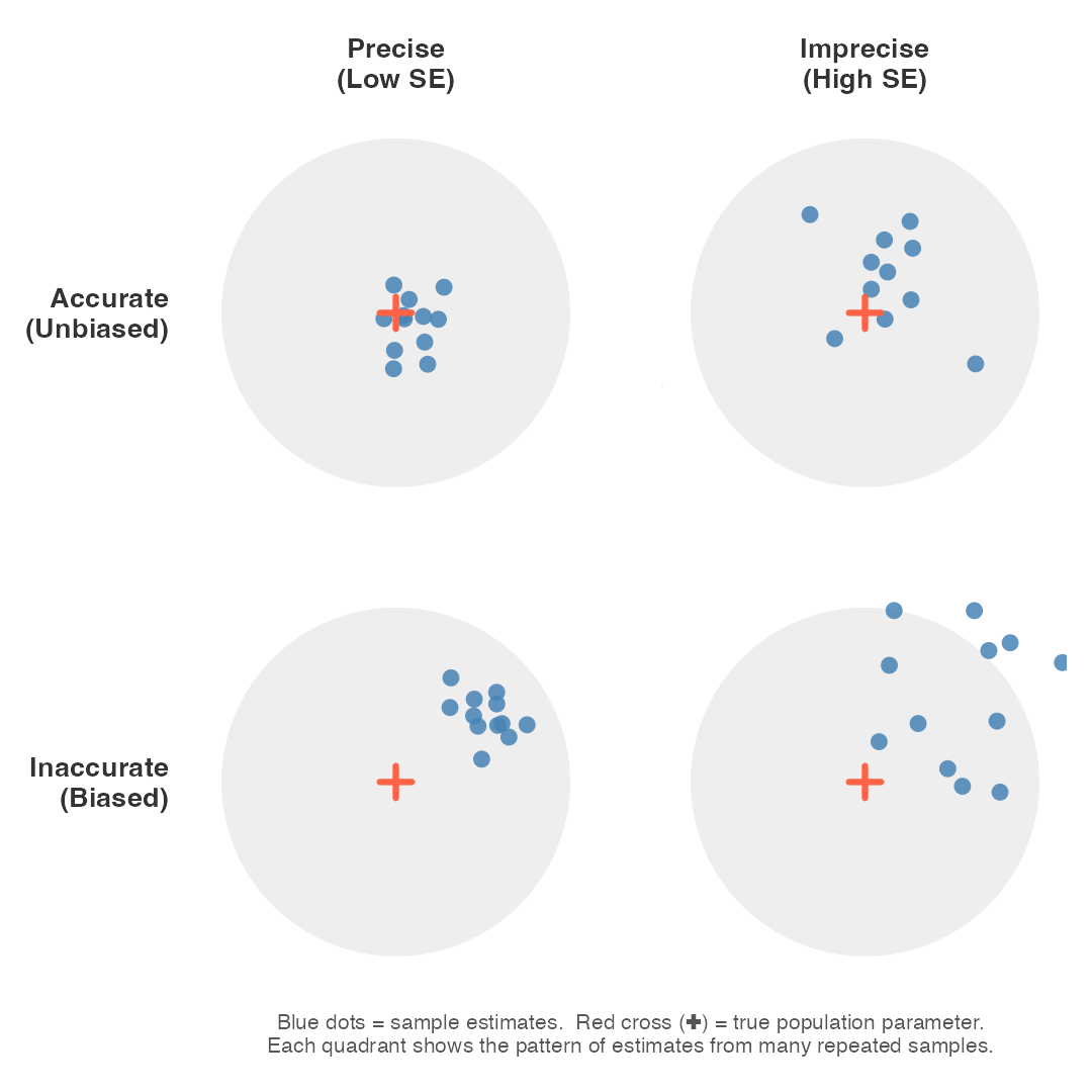
Each blue dot is one sample estimate; the red cross marks the true parameter. Top-left is the ideal: estimates cluster tightly around the truth.

The two are seperate concepts. An estimator can be accurate but imprecise (estimates scattered around the truth), or precise but inaccurate (estimates consistently off-target in the same direction). Generally, the precision of an estimator tends to improve as the sample size increases.

2.3.3 Shape

The shape of the sampling distribution is also important. It tells us a lot about the behavior of the statistic, can inform us about the probability of getting a sample mean in a certain range, and it can also help us determine which statistical methods are appropriate for inference.

What determines the shape of the sampling distribution? Two things: the shape of the population distribution and the sample size. For small samples, there’s not much we can say about the sampling distribution of $\bar{X}$, as it highly depends on the unknown population distribution. However, as the sample size grows, something remarkable happens: the sampling distribution becomes approximately bell-shaped, regardless of the shape of the population distribution. We’ll investigate this further in Module 3.

2.4 Effect of sample size

One of the most important practical questions in statistics is: how large does my sample need to be? Let’s investigate this directly by comparing the sampling distribution of $\bar{X}$ for different sample sizes.

{
  const mu = 1002.7;
  const sigma = 151.0;
  
  // Create container element
  const container = html`<div style="
    border: 1px solid #e2e8f0;
    border-radius: 12px;
    padding: 20px;
    background: #ffffff;
    box-shadow: 0 4px 6px -1px rgb(0 0 0 / 0.05), 0 2px 4px -2px rgb(0 0 0 / 0.05);
    max-width: 680px;
    margin: 15px auto;
    font-family: -apple-system, BlinkMacSystemFont, 'Segoe UI', Roboto, Helvetica, Arial, sans-serif;
  ">
    <!-- Header -->
    <div style="display: flex; justify-content: space-between; align-items: center; margin-bottom: 15px; border-bottom: 1px solid #f1f5f9; padding-bottom: 10px;">
      <span style="font-weight: 700; font-size: 16px; color: #1e293b;">Standard Error & Sample Size Simulator</span>
      <span style="font-size: 12px; color: #64748b; font-weight: 500;">Population: μ = 1002.7 psi, σ = 151.0 psi</span>
    </div>

    <!-- Dashboard Cards Grid: 2 columns for n and SE -->
    <div style="display: grid; grid-template-columns: repeat(2, 1fr); gap: 12px; margin-bottom: 15px;">
      <!-- Card 1: n -->
      <div style="background: #f8fafc; border: 1px solid #e2e8f0; border-radius: 8px; padding: 12px; text-align: center;">
        <div style="font-size: 11px; text-transform: uppercase; letter-spacing: 0.05em; color: #64748b; font-weight: 600; margin-bottom: 4px;">Sample Size (n)</div>
        <div id="sd-n-val" style="font-size: 24px; font-weight: 800; color: #0f172a;">200</div>
      </div>
      <!-- Card 2: SE -->
      <div style="background: #f0fdf4; border: 1px solid #bbf7d0; border-radius: 8px; padding: 12px; text-align: center;">
        <div style="font-size: 11px; text-transform: uppercase; letter-spacing: 0.05em; color: #166534; font-weight: 600; margin-bottom: 4px;">Standard Error (SE)</div>
        <div id="sd-se-val" style="font-size: 24px; font-weight: 800; color: #14532d;">10.7 psi</div>
      </div>
    </div>

    <!-- Controls Row -->
    <div style="background: #f8fafc; border: 1px solid #e2e8f0; border-radius: 8px; padding: 12px; margin-bottom: 15px;">
      <div style="display: flex; align-items: center; justify-content: space-between; margin-bottom: 8px; flex-wrap: wrap; gap: 8px;">
        <span style="font-size: 13px; font-weight: 600; color: #334155;">Adjust Sample Size (n):</span>
        <div style="display: flex; gap: 6px;">
          <button class="preset-btn" data-n="30" style="padding: 2px 8px; font-size: 11px; border: 1px solid #cbd5e1; background: #fff; border-radius: 4px; cursor: pointer; font-weight: 600; color: #475569; transition: all 0.2s;">n = 30</button>
          <button class="preset-btn" data-n="100" style="padding: 2px 8px; font-size: 11px; border: 1px solid #cbd5e1; background: #fff; border-radius: 4px; cursor: pointer; font-weight: 600; color: #475569; transition: all 0.2s;">n = 100</button>
          <button class="preset-btn" data-n="300" style="padding: 2px 8px; font-size: 11px; border: 1px solid #cbd5e1; background: #fff; border-radius: 4px; cursor: pointer; font-weight: 600; color: #475569; transition: all 0.2s;">n = 300</button>
          <button class="preset-btn" data-n="1000" style="padding: 2px 8px; font-size: 11px; border: 1px solid #cbd5e1; background: #fff; border-radius: 4px; cursor: pointer; font-weight: 600; color: #475569; transition: all 0.2s;">n = 1000</button>
          <button class="preset-btn" data-n="2000" style="padding: 2px 8px; font-size: 11px; border: 1px solid #cbd5e1; background: #fff; border-radius: 4px; cursor: pointer; font-weight: 600; color: #475569; transition: all 0.2s;">n = 2000</button>
        </div>
      </div>
      <div style="display: flex; align-items: center; gap: 10px;">
        <button id="slider-minus" style="padding: 2px 8px; border: 1px solid #cbd5e1; background: #fff; border-radius: 4px; cursor: pointer; font-weight: 700; color: #475569; width: 28px; height: 28px; display: flex; align-items: center; justify-content: center; font-size: 14px; user-select: none; transition: all 0.2s;">-</button>
        <input type="range" id="sd-slider" min="20" max="2000" step="10" value="200" style="flex-grow: 1; accent-color: #0284c7; cursor: pointer; height: 6px; border-radius: 3px; background: #cbd5e1;">
        <button id="slider-plus" style="padding: 2px 8px; border: 1px solid #cbd5e1; background: #fff; border-radius: 4px; cursor: pointer; font-weight: 700; color: #475569; width: 28px; height: 28px; display: flex; align-items: center; justify-content: center; font-size: 14px; user-select: none; transition: all 0.2s;">+</button>
      </div>
    </div>

    <!-- Plot Area -->
    <div id="sd-plot-container" style="display: flex; justify-content: center; min-height: 320px;"></div>
  </div>`;

  // Function to compute density values and generate the Plot
  function updatePlot(n) {
    const se = sigma / Math.sqrt(n);

    // Update stats text
    container.querySelector("#sd-n-val").textContent = n;
    container.querySelector("#sd-se-val").textContent = `${se.toFixed(1)} psi`;

    // Generate curves
    const xMin = 800;
    const xMax = 1200;
    const steps = 250;
    const stepSize = (xMax - xMin) / steps;
    
    const currentCurve = [];
    const refCurve = [];
    const se30 = sigma / Math.sqrt(30);

    for (let i = 0; i <= steps; i++) {
      const x = xMin + i * stepSize;
      
      const density = Math.exp(-Math.pow((x - mu), 2) / (2 * se * se)) / (se * Math.sqrt(2 * Math.PI));
      currentCurve.push({ x, density });

      const density30 = Math.exp(-Math.pow((x - mu), 2) / (2 * se30 * se30)) / (se30 * Math.sqrt(2 * Math.PI));
      refCurve.push({ x, density: density30 });
    }

    const maxDensity = Math.max(...currentCurve.map(d => d.density));
    const peak30 = 1 / (se30 * Math.sqrt(2 * Math.PI));
    const plotMaxY = Math.max(maxDensity, peak30);

    // Create plot
    const plotSvg = Plot.plot({
      style: {
        fontSize: "11px",
        fontFamily: "-apple-system, BlinkMacSystemFont, 'Segoe UI', Roboto, sans-serif"
      },
      width: 640,
      height: 320,
      grid: true,
      x: {
        label: "Sample Mean Crack Pressure (psi) →",
        domain: [800, 1200]
      },
      y: {
        label: "Probability Density",
        domain: [0, plotMaxY * 1.1] // Dynamic scaling to fit both curves without clipping at small n
      },
      marks: [
        Plot.ruleY([0], { stroke: "#cbd5e1" }),
        
        // Shaded area under current curve
        Plot.areaY(currentCurve, {
          x: "x",
          y1: 0,
          y2: "density",
          fill: "#0284c7",
          fillOpacity: 0.1
        }),

        // Baseline reference curve (n=30)
        Plot.line(refCurve, {
          x: "x",
          y: "density",
          stroke: "#94a3b8",
          strokeWidth: 1.5,
          strokeDasharray: "4 4"
        }),

        // Current sampling distribution curve
        Plot.line(currentCurve, {
          x: "x",
          y: "density",
          stroke: "#0284c7",
          strokeWidth: 2.5
        }),

        // Red dashed line for the population mean
        Plot.ruleX([mu], {
          stroke: "#ef4444",
          strokeWidth: 2,
          strokeDasharray: "4 2"
        }),

        // Mean label
        Plot.text(
          [{ x: mu, y: maxDensity * 1.03, text: `μ = ${mu.toFixed(1)} psi` }],
          { x: "x", y: "y", text: "text", fontSize: 11, fill: "#ef4444", textAnchor: "middle", fontWeight: "bold" }
        ),

        // Baseline label placed at a fixed height near the baseline curve shoulder
        Plot.text(
          [{ x: 940, y: 0.010, text: "Baseline (n = 30)" }],
          { x: "x", y: "y", text: "text", fontSize: 10, fill: "#64748b", textAnchor: "middle" }
        )
      ]
    });

    const plotContainer = container.querySelector("#sd-plot-container");
    plotContainer.innerHTML = "";
    plotContainer.appendChild(plotSvg);
  }

  // Helper to handle active preset highlighting
  const presetBtns = container.querySelectorAll(".preset-btn");
  function updatePresetHighlights(val) {
    presetBtns.forEach(btn => {
      if (+btn.getAttribute("data-n") === val) {
        btn.style.background = "#0284c7";
        btn.style.color = "#fff";
        btn.style.borderColor = "#0284c7";
      } else {
        btn.style.background = "#fff";
        btn.style.color = "#475569";
        btn.style.borderColor = "#cbd5e1";
      }
    });
  }

  // Set up event listeners
  const slider = container.querySelector("#sd-slider");
  slider.addEventListener("input", (e) => {
    const val = +e.target.value;
    updatePlot(val);
    updatePresetHighlights(val);
  });

  presetBtns.forEach(btn => {
    btn.addEventListener("click", () => {
      const val = +btn.getAttribute("data-n");
      slider.value = val;
      updatePlot(val);
      updatePresetHighlights(val);
    });
  });

  // Step change function for +/- buttons
  function changeVal(delta) {
    let val = +slider.value + delta;
    val = Math.max(+slider.min, Math.min(+slider.max, val));
    slider.value = val;
    updatePlot(val);
    updatePresetHighlights(val);
  }

  const minusBtn = container.querySelector("#slider-minus");
  const plusBtn = container.querySelector("#slider-plus");

  minusBtn.addEventListener("click", () => changeVal(-10));
  plusBtn.addEventListener("click", () => changeVal(10));

  // Add button hover transitions
  const addHover = (btn) => {
    btn.addEventListener("mouseenter", () => {
      btn.style.background = "#f1f5f9";
      btn.style.borderColor = "#94a3b8";
    });
    btn.addEventListener("mouseleave", () => {
      btn.style.background = "#fff";
      btn.style.borderColor = "#cbd5e1";
    });
  };
  addHover(minusBtn);
  addHover(plusBtn);

  // Set initial active state on n=200 preset if matched, otherwise no
  updatePlot(200);

  return container;
}

Figure 2.3: The sampling distribution of $\bar{X}$ for different sample sizes (population: screens_pop, $\mu = 1002.7$ psi, $\sigma = 151.0$ psi). As $n$ increases, the distribution narrows (i.e., estimates become more precise).

Exercise 2.3 (Explore: The Cost of Precision) Let’s investigate the relationship between sample size, standard error, and cost using the simulator in Figure 2.3. Suppose it costs $5 to collect and test each screen. Increasing the sample size by $400$ screens costs exactly $2,000 ($400 \times \$5$). Suppose you are willing to spend $2,000 to reduce the standard error of your estimate. How much precision do you actually get for your money?

Scenario A: Suppose your initial sample size is $n = 100$. You decide to increase it by $400$ screens to $n = 500$.
Scenario B: Suppose your initial sample size is $n = 1{,}500$. You decide to increase it by $400$ screens to $n = 1{,}900$.

In both scenarios, you increase the sample size by exactly 400 screens (spending exactly $2,000).

Which of the following statements best describes the trade-off of spending this $2,000?

viewof answer_dim_returns = Inputs.radio(
  [
    "We get the exact same gain in precision in both scenarios because we increase the sample size by 400.",
    "Scenario A is a much better investment, because spending $2,000 yields a large precision gain (8.3 psi), whereas in Scenario B, spending the same $2,000 yields an almost imperceptible gain (0.4 psi).",
    "Scenario B is a better investment, because larger sample sizes are always more precise so it is always worth spending more money.",
    "There is not enough information to answer this question. "
  ],
  {label: "Your answer: ", layout: "vertical", format: x => htl.html`<span style="display:inline-block; padding-bottom: 10px">${x}</span>`}
)

□

Exercise 2.3 demonstrates the law of diminishing returns in sampling. While larger samples are always more precise, the reward for increasing your sample size gets progressively smaller. Eventually, the financial or physical cost of collecting more data outweighs the tiny gain in precision. The implications of this are profound: when sampling, what matters is the absolute size of the sample, not its size relative to the population (provided the population is much larger than the sample). Once you have a sufficiently large sample, increasing it further yields very little gain in precision. This is why arguments like “only 5,000 people out of a population of 50 million were surveyed, so the results are not reliable” are statistically unfounded. In large populations, it is mostly the sample size that determines the precision, not the fraction of the population sampled.

2.5 The Estimator as a Random Variable

In Section 2.2, we simulated $5{,}000$ different samples of size $n = 300$ and watched the sample mean $\bar{X}$ vary from sample to sample. This behavior is what makes a statistic like $\bar{X}$ a random variable.

Definition 2.4 (Random Variable and Realization) A random variable is a quantity whose value is determined by the outcome of a random process. A specific observed value computed from a completed random process is called a realization (or observation).

This gives us an important conceptual distinction:

The Estimator (the rule “compute the sample mean from a random sample”) is the random variable (e.g., $\bar{X}$). We do not know its value in advance.
The Estimate (a specific observed value like $\bar{x} = 1{,}012$ psi) is a single, fixed realization of that random variable.
The Parameter (the truth) is a fixed constant describing the entire population and does not change when we draw a new sample.

Why does this matter? Because it dictates when probability statements are meaningful. Asking “what is the probability that the random variable $\bar{X}$ is within $20$ psi of the truth?” makes perfect sense, because $\bar{X}$ takes a different value each time. But asking “what is the probability that the true mean $\mu = 1{,}000$ psi?” is meaningless; $\mu$ is a fixed number, not a random variable. It either is $1{,}000$ psi or it is not; there is no probability involved.

Let’s put this distinction into practice.

Exercise 2.4 (Sorting Quantities: Random Variable vs. Fixed Constant) Verify if you can classify various statistical quantities based on whether they are random variables (changing from sample to sample) or fixed constants (properties of the design or population).

Play the categorization game below to test your understanding.

0 of 8 cards sorted

2.6 Exercises

Exercise 2.5 A public health researcher takes a random sample of $250$ adults to estimate the proportion who have been diagnosed with hypertension.

(a) Which of the following quantities is a random variable?

viewof answer_sd_rv_1_a = Inputs.radio(
  ["The true proportion of adults in the country with hypertension",
   "The sample proportion of adults with hypertension among the 250 surveyed",
   "The total number of adults in the country",
   "The sample size of 250"],
  {label: "Random variable: "}
)

(b) After completing the survey, the researcher reports: “In our sample, $22\%$ of participants have been diagnosed with hypertension.” Is this $22\%$ a random variable, or a realization of a random variable?

viewof answer_sd_rv_1_b = Inputs.radio(
  ["A random variable: it was computed from a random sample",
   "A realization of a random variable: it is one specific observed value",
   "Neither: it is just a summary statistic"],
  {label: "The 22%: "}
)

Exercise 2.6 Look back at the simulation in Section 2.2, where we took $5{,}000$ different samples of size $n = 300$ from screens_pop and plotted the resulting $\bar{X}$ values. Which of the following best describes what that histogram represents?

viewof answer_sd_rv_2 = Inputs.radio(
  ["The population distribution: how crack pressures are distributed across all 50,000 screens",
   "A sample distribution: the crack pressures within one specific sample of 300 screens",
   "The sampling distribution of X̄: the distribution of the random variable 'sample mean from 300 screens'",
   "The distribution of the fixed parameter μ"],
  {label: "That histogram represents: "}
)

Exercise 2.7 A regional hospital system recorded the time (in minutes) each patient spent waiting in the emergency department before being seen by a physician. Across $20{,}000$ visits logged last year, the wait time has a population mean of $\mu = 45$ minutes and a standard deviation of $\sigma = 20$ minutes.

We take $3{,}000$ random samples of size $n = 50$ and compute the sample mean for each. The results are stored in sampling_dist_wait.

(a) Simulate the sampling distribution of $\bar{X}$ with $n = 50$ and $3{,}000$ repetitions.

Hint

Use rep_sample_n() from the infer package. The first blank is the function name; the second and third are the size and reps arguments.

wait_time_pop |>
  rep_sample_n(size = ___, reps = ___) |>
  summarise(xbar = mean(wait_mins))

(b) Compute the mean and the standard error of the sampling distribution you created. Store them in a dataframe called summaries_sampling_dist. Compare the mean to the population mean.

summaries_sampling_dist <-
  sampling_dist_wait |>
    summarise(
      mean_xbar = mean(xbar),
      se_xbar   = sd(xbar)
    )

# Population mean
pop_mean_wait <- mean(wait_time_pop$wait_mins)

cat("Population mean:", pop_mean_wait, "\n")
cat("Mean of xbars:  ", summaries_sampling_dist$mean_xbar, "\n")

viewof answer_sd_3_1_c = Inputs.radio(
  ["The SE approximately doubled",
   "The SE approximately halved",
   "The SE approximately stayed the same",
   "The SE quadrupled"],
  {label: "What happened to the SE? "}
)

□

Exercise 2.8 Two researchers, Alice and Bob, study the same population. Alice uses samples of size $n = 100$ and Bob uses samples of size $n = 400$.

(a) Who has the smaller standard error?

viewof answer_sd_3_2_a = Inputs.radio(
  ["Alice",
   "Bob",
   "They are the same",
   "Impossible to tell without more information"],
  {label: "Who has the smaller SE? "}
)

□

Exercise 2.9 A real estate platform recorded the sale prices (in thousands of dollars) for $25{,}000$ homes sold in a major Canadian city last year. The data are stored in home_sales_pop.

(a) Is the population distribution symmetric, left-skewed, or right-skewed?

viewof answer_sd_3_3_a = Inputs.radio(
  ["Symmetric",
   "Left-skewed (long tail to the left)",
   "Right-skewed (long tail to the right)"],
  {label: "Shape: "}
)

(b) Simulate the sampling distribution of the sample median for samples of size $n = 40$ with $3{,}000$ repetitions.

set.seed(20)
sampling_dist_median <-
  home_sales_pop |>
  rep_sample_n(size = 40, reps = 3000) |>
  summarise(med = median(price_k))

sampling_dist_median |>
  ggplot(aes(x = med)) +
  geom_histogram(bins = 40, fill = "coral", color = "white") +
  labs(
    title = "Sampling distribution of the sample median (n = 40)",
    x     = "Sample median price (thousands of dollars)",
    y     = "Count"
  ) +
  theme_classic()

□

With the help of the surreal approach, we have now explored sampling distribution and its role in statistical inference. However, as the name suggests, the surreal approach is not viable in practice because we never have access to the entire population. In a real study, you have exactly one sample, and there is no going back to the population for more.

Yet everything we have built here still applies. The sampling distribution describes how much an estimate typically varies from the truth, and that description is precisely what we need to quantify uncertainty and draw reliable conclusions. The challenge that remains is approximating the sampling distribution from the single sample we actually have, without the population in hand. There are two principled paths forward: bootstrapping, which uses the sample itself to simulate the sampling process, and the Central Limit Theorem, which provides a mathematical description of the sampling distribution through theory alone. Together, they transform the concepts of this tutorial into the everyday tools of statistical inference. We will start next with bootstrapping in Chapter 2.

2.7 Take-home points

The population distribution (fixed, usually unknown), the sample distribution (observable, changes with each new sample), and the sampling distribution (describes how a statistic varies across all possible samples of size $n$) are three distinct and important concepts that are easy to confuse.
Sampling variability: the fact that different random samples produce different statistics, is the reason a single estimate cannot be blindly trusted. The sampling distribution of a statistic quantifies exactly how much that estimate could plausibly vary, which is what lets us judge how trustworthy it is.
The sampling distribution of a statistic describes how the statistic varies across all possible samples of size $n$. Two key properties:
- Center: A statistic is unbiased if the mean of its sampling distribution equals the true population parameter; it gets the right answer on average, even though any single estimate will typically differ from the truth.
- Spread: The standard error (SE) is the standard deviation of the sampling distribution. Larger sample sizes ($n$) yield smaller standard errors and more precise estimates, but with diminishing returns: to halve the standard error, you must quadruple the sample size.
Even with access to the population, the sampling distribution cannot be calculated directly; we can only approximate it via the surreal approach (drawing many samples and computing the statistic for each). In practice, however, we never have access to the entire population, so we must approximate it from the single sample we have. The two main ways to do this are Bootstrapping and the Central Limit Theorem.
Key R function: rep_sample_n(size = n, reps = B, replace = FALSE) from the infer package draws $B$ independent random samples of size $n$ from a data frame, with or without replacement. Paired with summarise(), it is the main tool for simulating a sampling distribution in this course.