Multiple Linear Regression

STAT 306 - Module 08

Learning objectives

Express a multiple linear regression model in matrix form, defining all vectors and matrices involved.
Provide the dimensions of all vectors and matrices relevant to a multiple linear regression model.
Define key statistics that can be computed in the fit of a linear model, including the residual sum of squares, the residual mean square, \(R^{2}\), and adjusted \(R^2\), in terms of vectors and matrices.
Explain how the residual sum of squares, the residual mean square, \(R^{2}\), and adjusted \(R^{2}\) can vary with the addition of explanatory variables to the fitted linear model.

Multiple Linear Regression: our goals for upcoming lectures

What are the least squares estimators and their properties?
What changes in the interpretation of such models, or when making inference/predictions with them?
Confidence intervals and hypothesis tests for the parameters.
Prediction intervals for future observations.
Model diagnostics.

The MLR model

Suppose we want to explain \(Y\) using \(p\) covariates \(X_1, \ldots, X_p\).
The model generalizes very naturally to: \[ Y_i = \beta_0 + \beta_1X_{i1} + \cdots + \beta_pX_{ip} + \varepsilon_i \;,\quad i=1,\ldots,n \;, \]

In matrix form: \[ \mathbf{Y} = \mathbf{X}\pmb{\beta} + \pmb{\varepsilon} \;, \] where:

\[ \mathbf{Y} = \begin{bmatrix} Y_1 \\ Y_2 \\ \vdots \\ Y_n \end{bmatrix}_{n \times 1} \;, \ \mathbf{X} = \begin{bmatrix} 1 & x_{11} & x_{12} & \cdots & x_{1p} \\ 1 & x_{21} & x_{22} & \cdots & x_{2p} \\ \vdots & \vdots & \vdots & \ddots & \vdots \\ 1 & x_{n1} & x_{n2} & \cdots & x_{np} \end{bmatrix}_{n \times (p+1)} \;, \\ \pmb{\beta} = \begin{bmatrix} \beta_0 \\ \beta_1 \\ \vdots \\ \beta_p \end{bmatrix}_{(p+1) \times 1} \;, \ \pmb{\varepsilon} = \begin{bmatrix} \varepsilon_1 \\ \varepsilon_2 \\ \vdots \\ \varepsilon_n \end{bmatrix}_{n \times 1} \;. \]

A linear model is any model that can be written in the form \[ \mathbf{Y} = \mathbf{X}\pmb{\beta} + \pmb{\varepsilon} \;. \]

iClicker 1

Which of the following models is a linear model?

\(Y_i = \beta_0 + \beta_1x_{i1} + e^{\beta_2x_{i2}} + \varepsilon_i\)
\(Y_i = \beta_0 + \beta_1x_{i1} + \beta_2x_{i1}^2 + \varepsilon_i\)
\(Y_i = \beta_0 + \beta_1x_{i1} + \dfrac{\beta_2}{\beta_1}x_{i1}^2 + \varepsilon_i\)
\(Y_i = \beta_0 + \beta_1x_{i1} + \log(\beta_2x_{i2}) + \varepsilon_i\)

iClicker 1: Solution

Which of the following models is a linear model?

\(Y_i = \beta_0 + \beta_1x_{i1} + e^{\beta_2x_{i2}} + \varepsilon_i\)
\(Y_i = \beta_0 + \beta_1x_{i1} + \beta_2x_{i1}^2 + \varepsilon_i\)
\(Y_i = \beta_0 + \beta_1x_{i1} + \dfrac{\beta_2}{\beta_1}x_{i1}^2 + \varepsilon_i\)
\(Y_i = \beta_0 + \beta_1x_{i1} + \log(\beta_2x_{i2}) + \varepsilon_i\)

Hyperplane

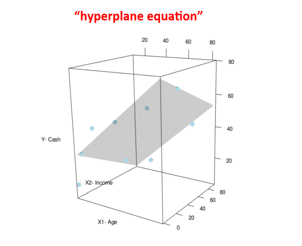
Note that if we have more than one covariate (i.e., \(p>1\)), then \((X_1,\dots,X_p,Y)\) lives in a \((p+1)\)-dimensional space.
We don’t have a line anymore: the regression surface is a \(p\)-dimensional hyperplane inside that \((p+1)\)-dimensional space.

The residuals in matrix form

The residuals of a model with coefficients \(\mathbf{b}^\top=\left[b_0, b_1, ..., b_p\right]\) are given by: \[ \mathbf{e} = \mathbf{Y} - \mathbf{X}\mathbf{b} \]

iClicker 2

To fit the model \(\mathbf{Y} = \mathbf{X}\pmb{\beta} + \pmb{\varepsilon}\) we minimize the residual sum of squares \(RSS(\mathbf{b}) = \sum_{i=1}^n e_i^2\), which can be written as

\(\mathbf{e}\mathbf{e}^\top\)
\(\mathbf{e}^\top\mathbf{e}\)
\(\sum_{i=1}^n \mathbf{e}^\top\mathbf{e}\)
\(\sum_{i=1}^n \mathbf{e}\mathbf{e}^\top\)
\(\sum_{i=1}^n \mathbf{e}^2\)

iClicker 2: Solution

To fit the model \(\mathbf{Y} = \mathbf{X}\pmb{\beta} + \pmb{\varepsilon}\) we minimize the residual sum of squares \(RSS(\mathbf{b}) = \sum_{i=1}^n e_i^2\), which can be written as

\(\mathbf{e}\mathbf{e}^\top\)
\(\mathbf{e}^\top\mathbf{e}\)
\(\sum_{i=1}^n \mathbf{e}^\top\mathbf{e}\)
\(\sum_{i=1}^n \mathbf{e}\mathbf{e}^\top\)
\(\sum_{i=1}^n \mathbf{e}^2\)

RSS in matrix form

The Residual Sum of Squares (RSS) of a model with coefficients \(\mathbf{b}^\top=\left[b_0, b_1, ..., b_p\right]\) is given by: \[ RSS(\mathbf{b}) = \sum_{i=1}^n e_i^2 = \begin{bmatrix} e_1 & e_2 & \ldots & e_n \end{bmatrix} \begin{bmatrix} e_1 \\ e_2 \\ \vdots \\ e_n \end{bmatrix} = \mathbf{e}^\top\mathbf{e} \]

Estimator of the variance of the errors

For SLR, since we had only two coefficients, we used the estimator of the variance of the errors \[ \hat{\sigma}^2 = \frac{RSS}{n-2} \]
For MLR, since we have \(p+1\) coefficients, we use \[ \hat{\sigma}^2 = \frac{RSS}{n-(p+1)} \]

Fitting the MLR Model

Matrix calculus: cheatsheet

Let \(\mathbf{a}\) and \(\mathbf{y}\) be two \(p\)-dimensional vectors.
- \(\frac{\partial \mathbf{a}^\top\mathbf{y}}{\partial \mathbf{y}} = \frac{\partial \mathbf{y}^\top\mathbf{a}}{\partial \mathbf{y}} = \mathbf{a}\)
- \(\frac{\partial \mathbf{y}^\top\mathbf{y}}{\partial \mathbf{y}} = 2\mathbf{y}\)
- \(\frac{\partial \mathbf{y}^\top\mathbf{B}\mathbf{y}}{\partial \mathbf{y}} = \left(\mathbf{B} + \mathbf{B}^\top\right)\mathbf{y}\)
- \(\frac{\partial \mathbf{y}^\top\mathbf{B}\mathbf{a}}{\partial \mathbf{y}} = \mathbf{B}\mathbf{a}\)

Activity: Minimizing SSR

Minimize the \(RSS(\mathbf{b}) = \mathbf{e}^\top\mathbf{e}\) to obtain the least squares estimator \(\widehat{\pmb{\beta}}\) of the coefficients \(\pmb{\beta}\).

We want to find the coefficients \(\widehat{\pmb{\beta}}\) that minimize the RSS

\[ \begin{align} RSS(\mathbf{b}) &= \mathbf{e}^\top\mathbf{e}\\ &= (\mathbf{Y} - \mathbf{X}\mathbf{b})^\top(\mathbf{Y} - \mathbf{X}\mathbf{b}) \\ &= \mathbf{b}^\top\mathbf{X}^\top\mathbf{X}\mathbf{b} - \mathbf{b}^\top\mathbf{X}^\top\mathbf{Y} - \mathbf{Y}^\top\mathbf{X}\mathbf{b} + \mathbf{Y}^\top\mathbf{Y} \\ &= \mathbf{b}^\top\mathbf{X}^\top\mathbf{X}\mathbf{b} - 2\mathbf{b}^\top\mathbf{X}^\top\mathbf{Y} + \mathbf{Y}^\top\mathbf{Y} \end{align} \]

Then, we can take the derivative of \(RSS(\mathbf{b})\) with respect to \(\mathbf{b}\) and set it equal to zero to find the minimum.

\[ \frac{\partial RSS(\mathbf{b})}{\partial \mathbf{b}} = 2\mathbf{X}^\top\mathbf{X}\mathbf{b} - 2\mathbf{X}^\top\mathbf{Y} \]

Setting it to zero, we get \[ \begin{align} 2\mathbf{X}^\top\mathbf{X}\widehat{\pmb{\beta}} - 2\mathbf{X}^\top\mathbf{Y} &= 0\\ \mathbf{X}^\top\mathbf{X}\widehat{\pmb{\beta}} &= \mathbf{X}^\top\mathbf{Y} \end{align} \] which has the same form as the normal equation we obtained for simple linear regression.
If \(\mathbf{X}^\top\mathbf{X}\) is invertible, the unique least squares estimator is: \[ \widehat{\pmb{\beta}} = (\mathbf{X}^\top\mathbf{X})^{-1}\mathbf{X}^\top\mathbf{Y} \;. \]

Conditions for Invertibility in MLR

For a multiple linear regression model with \(p\) covariates, the design matrix \(\mathbf{X}\) is of dimension \(n \times (p+1)\).
The \((p+1) \times (p+1)\) matrix \(\mathbf{X}^\top\mathbf{X}\) is invertible if and only if \(\mathbf{X}\) has full column rank: \[ \operatorname{rank}(\mathbf{X}) = p+1 \]

In other words:
- The columns of \(\mathbf{X}\) must be linearly independent (no covariate is an exact linear combination of the other covariates).
- The sample size must be at least as large as the number of parameters: \(n \ge p+1\).
If \(\mathbf{X}^\top\mathbf{X}\) is singular (e.g., exact collinearity or \(n < p+1\)), the normal equations still have solutions, but the parameter estimate is not unique.

Activity

Suppose we want to explain penguins’ body mass not only by their flipper length but also by their bill length. Our linear model is then

\[ Y_i = \beta_0 + \beta_1x_{i1} +\beta_2x_{i2} +\varepsilon_i \;, \qquad \varepsilon_i\sim N(0,\sigma^2) \;. \]

Question 1

Construct the design matrix \(\mathbf{X}\) by completing the partial R code below. Which of the following R functions will you need to use to do so?

c()
rbind()
cbind()
data.frame()

Question 2

Some commands you’ll need to compute the least squares estimate \(\widehat{\pmb{\beta}}\):

The function t(A) computes the matrix transpose \(\mathbf{A}^\top\).
The operator A %*% B computes the matrix product \(\mathbf{AB}\).
The function solve(A,b) computes the vector c such that \(\mathbf{Ac=b}\).

Given the above, compute the least squares estimate

\[ \widehat{\pmb{\beta}} = (\mathbf{X}^\top\mathbf{X})^{-1}\mathbf{X}^\top\mathbf{y} \;. \]

iClicker 3

What is the least squares estimate of the coefficient parameter for bill_length_mm?

-5836.299
48.890
4.959
16.677
17.421

iClicker 3: Solution

What is the least squares estimate of the coefficient parameter for bill_length_mm?

-5836.299
48.890
4.959
16.677
17.421

Fitting with R

To fit a multiple linear regression model in R, use lm() and separate the covariates on the right-hand side of the formula with +.

The fitted regression equation is

\[ \widehat{\text{body mass}} = -5836.30 + 48.89\,(\text{flipper length}) + 4.96\,(\text{bill length}). \]

Interpretation of the coefficients

Each slope gives the expected change in the response for a one-unit increase in that covariate, keeping all other variables in the model constant.
Flipper-length coefficient (\(\widehat{\beta}_1 = 48.89\)):
- Keeping bill length constant, a 1 mm increase in flipper length is associated with an expected increase of \(48.89\text{ g}\) in body mass.
Bill-length coefficient (\(\widehat{\beta}_2 = 4.96\)):
- Keeping flipper length constant, a \(1\text{ mm}\) increase in bill length is associated with an expected increase of \(4.96\text{ g}\) in body mass.
Intercept (\(\widehat{\beta}_0 = -5836.30\)):
- The expected body mass for a penguin with flipper length and bill length both equal to zero. This is an extrapolation and has no meaningful physical interpretation in this case.

Important: Association is not causality.

Each slope describes an association with the response while the other covariates in the model are held fixed. It does not establish that changing a covariate causes body mass to change.

Question 3

Consider a model with two covariates, \(X_1\) and \(X_2\).
- You fitted the model and obtained a certain \(RSS(\hat\beta_0,\hat\beta_1,\hat\beta_2) = RSS_{p=2}\).
Later, you decided to add a third covariate \(X_3\) to the model.
- You fitted the new model and obtained a certain \(RSS(\hat\beta_0,\hat\beta_1,\hat\beta_2,\hat\beta_3) = RSS_{p=3}\).
Is there a relationship between \(RSS_{p=2}\) and \(RSS_{p=3}\)?

iClicker 4

What is the relationship between \(RSS_{p=2}\) and \(RSS_{p=3}\)?

\(\min RSS_{p=2} = \min RSS_{p=3}\)
\(\min RSS_{p=2} \geq \min RSS_{p=3}\)
\(\min RSS_{p=2} \leq \min RSS_{p=3}\)
We can’t guarantee any of the above.

iClicker 4: Solution

What is the relationship between \(RSS_{p=2}\) and \(RSS_{p=3}\)?

\(\min RSS_{p=2} = \min RSS_{p=3}\)
\(\min RSS_{p=2} \geq \min RSS_{p=3}\)
\(\min RSS_{p=2} \leq \min RSS_{p=3}\)
We can’t guarantee any of the above.

Question 3: Solution

Consider a model with two covariates, \(X_1\) and \(X_2\).
- You fitted the model and obtained a certain \(RSS(\hat\beta_0,\hat\beta_1,\hat\beta_2) = RSS_{p=2}\).
Later, you decided to add a third covariate \(X_3\) to the model.
- You fitted the new model and obtained a certain \(RSS(\hat\beta_0,\hat\beta_1,\hat\beta_2,\hat\beta_3) = RSS_{p=3}\).
Is there a relationship between \(RSS_{p=2}\) and \(RSS_{p=3}\)?

Solution

Just note that the solution \(\widehat{\pmb{\beta}}\) for the \(p=2\) model is a valid solution for the \(p=3\) model.
- If we set \(b_3=0\), then the \(p=3\) model reduces to the \(p=2\) model.
Hence, the minimum value of \(RSS\) for the \(p=3\) model must be less than or equal to that for the \(p=2\) model.
In other words, adding covariates to our linear model never increases the minimum value achievable for the residual sum of squares (which is a measure of the “error” made by the model on our data).
Does this mean we should always add as many variables as we can to our model?
- NO!

Question 4

Our estimator of \(\sigma^2\), the residual mean square \(\hat{\sigma}^2\), is defined as \[ \hat{\sigma}^2 = \frac{\mathbf{e}^\top\mathbf{e}}{n-(p+1)} = \frac{RSS}{n-(p+1)} \;. \]
Suppose that \(0<R^2<1\) and we add an additional covariate to the model.
1. How could the coefficient of determination \(R^2\) change?
2. How could the residual mean square \(\hat{\sigma}^2\) change?

iClicker 5

Knowing that \(\min RSS_{p=2} \geq \min RSS_{p=3}\), what can we say about \(R^2\) and \(\hat{\sigma}^2\) when we add a new covariate to a model?

\(R^2\) cannot increase, \(\hat{\sigma}^2\) cannot increase.
\(R^2\) cannot increase, \(\hat{\sigma}^2\) cannot decrease.
\(R^2\) cannot decrease, \(\hat{\sigma}^2\) cannot increase.
\(R^2\) cannot decrease, \(\hat{\sigma}^2\) cannot decrease.
\(R^2\) cannot decrease, \(\hat{\sigma}^2\) can increase or decrease.

iClicker 5: Solution

Knowing that \(\min RSS_{p=2} \geq \min RSS_{p=3}\), what can we say about \(R^2\) and \(\hat{\sigma}^2\) when we add a new covariate to a model?

\(R^2\) cannot increase, \(\hat{\sigma}^2\) cannot increase.
\(R^2\) cannot increase, \(\hat{\sigma}^2\) cannot decrease.
\(R^2\) cannot decrease, \(\hat{\sigma}^2\) cannot increase.
\(R^2\) cannot decrease, \(\hat{\sigma}^2\) cannot decrease.
\(R^2\) cannot decrease, \(\hat{\sigma}^2\) can increase or decrease.

Question 4: Solution

Our estimator of \(\sigma^2\), the residual mean square \(\hat{\sigma}^2\), is defined as \[ \hat{\sigma}^2 = \frac{\mathbf{e}^\top\mathbf{e}}{n-(p+1)} = \frac{RSS}{n-(p+1)} \;. \]
Suppose that \(0<R^2<1\) and we add an additional covariate to the model.
1. How could the coefficient of determination \(R^2\) change?
2. How could the residual mean square \(\hat{\sigma}^2\) change?

Solution

About \(R^2\), recall (Module 06) that \(TSS = \mathbf{y}^\top\mathbf{y}-n\bar{y}^2\) and \[ R^2 = 1 - \frac{RSS}{TSS} \]
\(TSS\) is fixed given the data, and as we saw in Question 3, adding covariates never increases \(RSS\). Hence, \(R^2\) will never decrease with additional covariates.
- This is a big deal because it means that \(R^2\) is not a good measure to compare models with different numbers of covariates.
About \(\hat{\sigma}^2\): \[ \hat{\sigma}^2 = \frac{RSS}{n-(p+1)} \]
With \(\hat\sigma^2\), the numerator \(RSS\) never increases with additional covariates. However, the denominator \(n-(p+1)\) decreases with additional covariates, and so it is possible that \(\hat\sigma^2\) may increase.

Adjusted \(R^2\)

To account for the number of predictors in the model, we can use the adjusted \(R^2\), which is \(R^2\) “corrected” for degrees of freedom and defined as \[ \mathrm{adj}\: R^2 = 1 - \frac{\left(\frac{RSS}{n-(p+1)}\right)}{\left(\frac{TSS}{n-1}\right)} = 1 - \frac{(n-1)\hat\sigma^2}{TSS} \;. \]
Unlike \(R^2\), adjusted \(R^2\) could increase, decrease, or stay unchanged with additional covariates. However, it is not lower-bounded by zero.
Both \(R^2\) and adjusted \(R^2\) are provided as output of summary().

What We Learned

MLR Model in Matrix Form: \[\mathbf{Y} = \mathbf{X}\pmb{\beta} + \pmb{\varepsilon}\]
- \(\mathbf{Y}_{n \times 1}\), \(\pmb{\varepsilon}_{n \times 1}\): response and error vectors.
- \(\mathbf{X}_{n \times (p+1)}\): design matrix, with a column of \(1\)’s for the intercept and one column per covariate.
- \(\pmb{\beta}_{(p+1) \times 1} = \begin{bmatrix} \beta_0 & \beta_1 & \cdots & \beta_p \end{bmatrix}^\top\): vector of parameters.
- A model is linear when it can be written this way, i.e., linear in \(\pmb{\beta}\).
Least Squares Estimate: minimizing \[RSS(\mathbf{b}) = \mathbf{e}^\top\mathbf{e} = (\mathbf{Y}-\mathbf{X}\mathbf{b})^\top(\mathbf{Y}-\mathbf{X}\mathbf{b})\] gives the same normal-equation form as in SLR, \[\mathbf{X}^\top\mathbf{X}\widehat{\pmb{\beta}} = \mathbf{X}^\top\mathbf{Y} \;,\] with unique solution \[\widehat{\pmb{\beta}} = (\mathbf{X}^\top\mathbf{X})^{-1}\mathbf{X}^\top\mathbf{Y}\] whenever \(\mathbf{X}^\top\mathbf{X}\) is invertible.
Invertibility: \(\mathbf{X}^\top\mathbf{X}\) is invertible if and only if \(\mathbf{X}\) has full column rank, \(\operatorname{rank}(\mathbf{X}) = p+1\):
- No column of \(\mathbf{X}\) (including the intercept) is an exact linear combination of the others.
- \(n \ge p+1\) (necessary, not sufficient).
Adding covariates never increases \(RSS\): the parameter space of a \(p\)-covariate model embeds in that of a \((p{+}1)\)-covariate model (by setting the new coefficient to \(0\)), so minimizing over the larger space can only match or beat the smaller one: \[ RSS_{p+1} \le RSS_p \;.\]
Consequences for model-fit statistics, with \(TSS = \mathbf{y}^\top\mathbf{y}-n\bar y^2\) fixed by the data:
- \(\hat\sigma^2 = \dfrac{RSS}{n-(p+1)}\): numerator never increases, but \(n-(p+1)\) shrinks, so \(\hat\sigma^2\) can increase or decrease.
- \(R^2 = 1-\dfrac{RSS}{TSS}\): never decreases — so \(R^2\) alone is not a good way to compare models with different numbers of covariates.
- adjusted \(R^2 = 1-\dfrac{(n-1)\hat\sigma^2}{TSS}\): can increase, decrease, or stay unchanged, and (unlike \(R^2\)) is not lower-bounded by \(0\).