SLR: Model Diagnostics and Final Remarks

STAT 306 - Module 06

Learning Objectives

  • By the end of this lecture, you should be able to:
    • Explain why residuals, not the response, are used to check the model assumptions, and state the constraints that the residuals satisfy.
    • Use residual-vs-fitted plots to detect non-linearity and heteroscedasticity.
    • Use a normal quantile plot to assess normality, and a plot of \(e_{i+1}\) against \(e_i\) (or of residuals against observation order) to detect serial correlation.
    • Prove the decomposition \(TSS = MSS + RSS\) and define \(R^2\) as the proportion of variability in \(Y\) explained by the model.
    • Explain why a high or low \(R^2\) does not by itself tell us whether the model is appropriate, or whether \(X\) and \(Y\) are related.
    • Explain what “linear” means in a linear model (linear in the parameters), and recognize how a lurking variable can reverse an association (Simpson’s paradox).

Simple linear model: Review

  • Given data \((x_i,y_i)\), \(i=1,\dotsc,n\), we could consider a linear model of the form \[ Y_i = \beta_0 + \beta_1x_i + \varepsilon_i \;, \qquad \varepsilon_i\overset{\text{iid}}{\sim} N(0,\sigma^2) \;, \] where \(\beta_0\) and \(\beta_1\) are unknown parameters and \(x_1,\dotsc,x_n\) are non-random.
  • The assumptions for the errors \(\varepsilon_i\) are:
    • It has a distribution:
      • We will assume it to be Normal;
    • It has a mean:
      • safely assumed to be 0 (i.e., \(\mathbb{E}[\varepsilon_i] = 0\));
    • It has a variance:
      • unknown and denoted by \(\sigma^2\) (i.e., \(Var(\varepsilon_i) = \sigma^2\));
    • The errors are independent of each other (in particular, \(Cov(\varepsilon_i, \varepsilon_j) = 0\) for \(i \neq j\)).
  • Fitting the model means finding estimates \(\hat{\beta}_0\) and \(\hat{\beta}_1\), which we can then use to obtain fitted values \[ \hat{y}_i = \hat\beta_0 + \hat\beta_1x_i \;, \qquad i = 1,\dotsc,n \;. \]
  • The residuals \(e_1,\dotsc,e_n\) of the model are the differences between the observed responses and the fitted values: \[ e_i = y_i - \hat{y}_i \;,\qquad i = 1,\dotsc,n \;. \]

Model Diagnostics

Diagnostics via residuals

  • There’s no guarantee that the model assumptions are reasonable for the data at hand.

  • Using \(Y\) to check the assumptions is hard because \(Y\) contains both the signal (the linear part) and the noise (the errors).

  • But if the model is appropriate (i.e., the assumptions are reasonable), then the errors \(\varepsilon_i\) should behave like i.i.d. observations from \(N(0,\sigma^2)\).

  • Unfortunately, the errors are not observable, so we use the residuals \(e_i\) as a proxy for the errors \(\varepsilon_i\).

Properties of residuals

  • The residuals have two constraints (which the errors do not have):
    1. \[ \sum_{i=1}^n e_i = 0 \;. \]

    2. \[ \sum_{i=1}^n x_i e_i = 0 \;. \]

  • Note that the first constraint means that the residuals always have a mean of \(0\).
    • Therefore, the sample mean of the residuals is not useful for checking the assumption \(\mathbb{E}[\varepsilon_i] = 0\).
  • However, when the sample size is large in comparison to the number of parameters, the residuals behave similarly to the errors.

Model diagnostics via residual plots

  • Residuals are often used for model diagnostics, i.e., to assess how well the model fits the data.

  • Several model diagnostic methods use plots to graphically determine if the observed residuals behave in ways that differ from how they should behave (in theory) under the model assumptions.

  • Some common plots include:

    1. \(e_i\) against the fitted value \(\hat{y}_i\) (or \(e_i\) against the covariate \(x_i\))
    2. ordered residual \(e_{(i)}\) against the normal score \(\mathbb{E}[z_{(i)}]\) (called a normal quantile plot), and
    3. \(e_i\) against \(e_{i-1}\) (or \(e_{i-2}\), etc.) for examining serial correlation.

Residuals vs fitted value (or covariate)

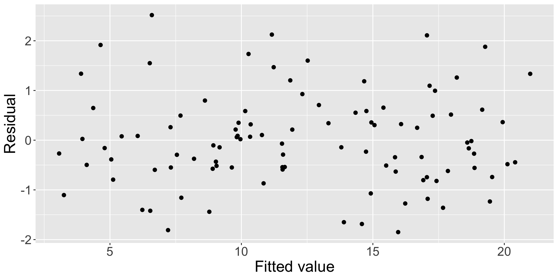
  • When the model fits well, the residuals should be (approximately) independent of the fitted value/covariate.
  • This means that the plots of
    1. \(e_i\) against the fitted value \(\hat{y}_i\), or
    2. \(e_i\) against the covariate \(x_i\)
    should not show any obvious pattern in the points, which are centered around zero.
  • Example of a residual-vs-fitted value plot for data generated from a linear model.
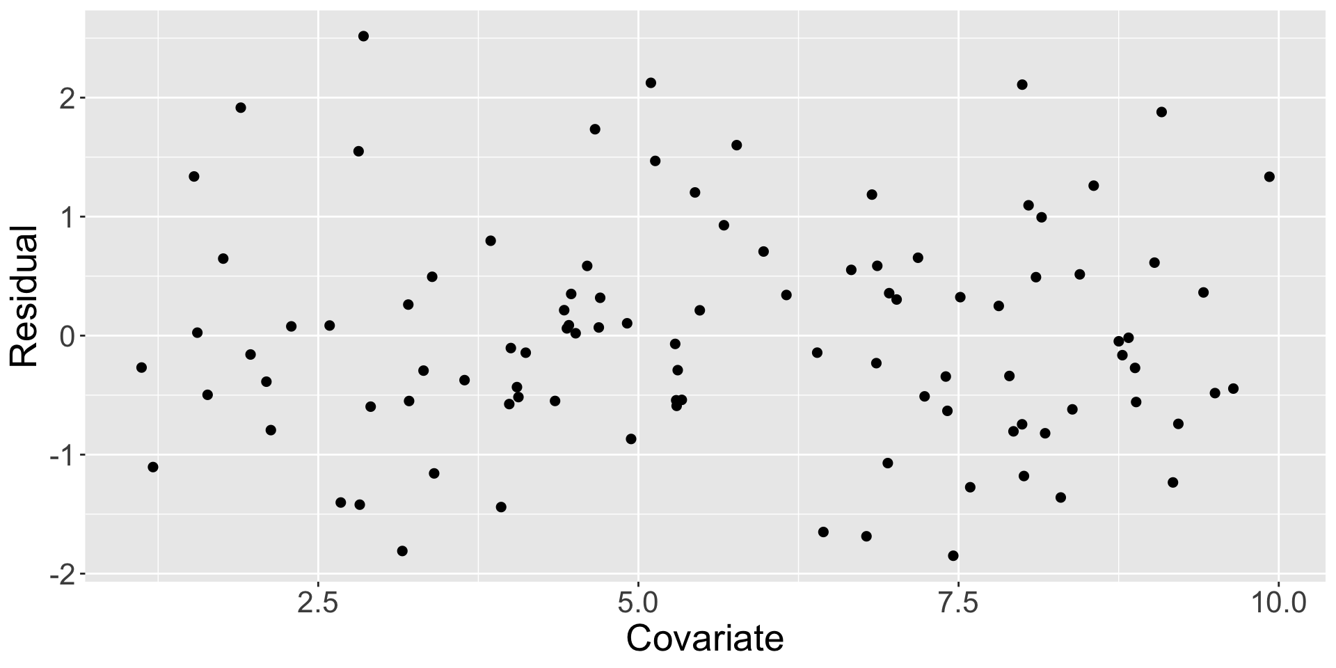
  • Note, the plot of \(e_i\) against \(x_i\) is equivalent to the above plot because \(\hat{y}_i = \hat\beta_0 + \hat\beta_1 x_i\) is a linear function of \(x_i\).
    • Just the scale and location of the \(x\)-axis are different, but the shape of the plot is the same.
Residuals vs fitted value: Nonlinearity

Scroll down

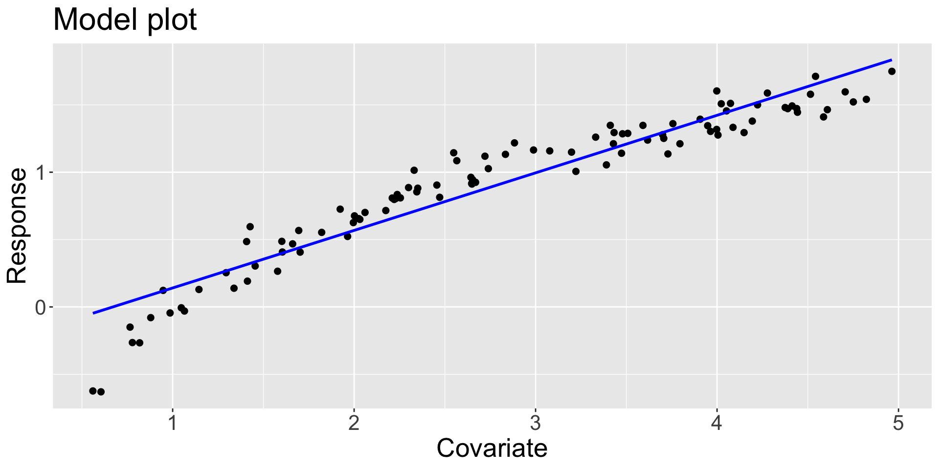
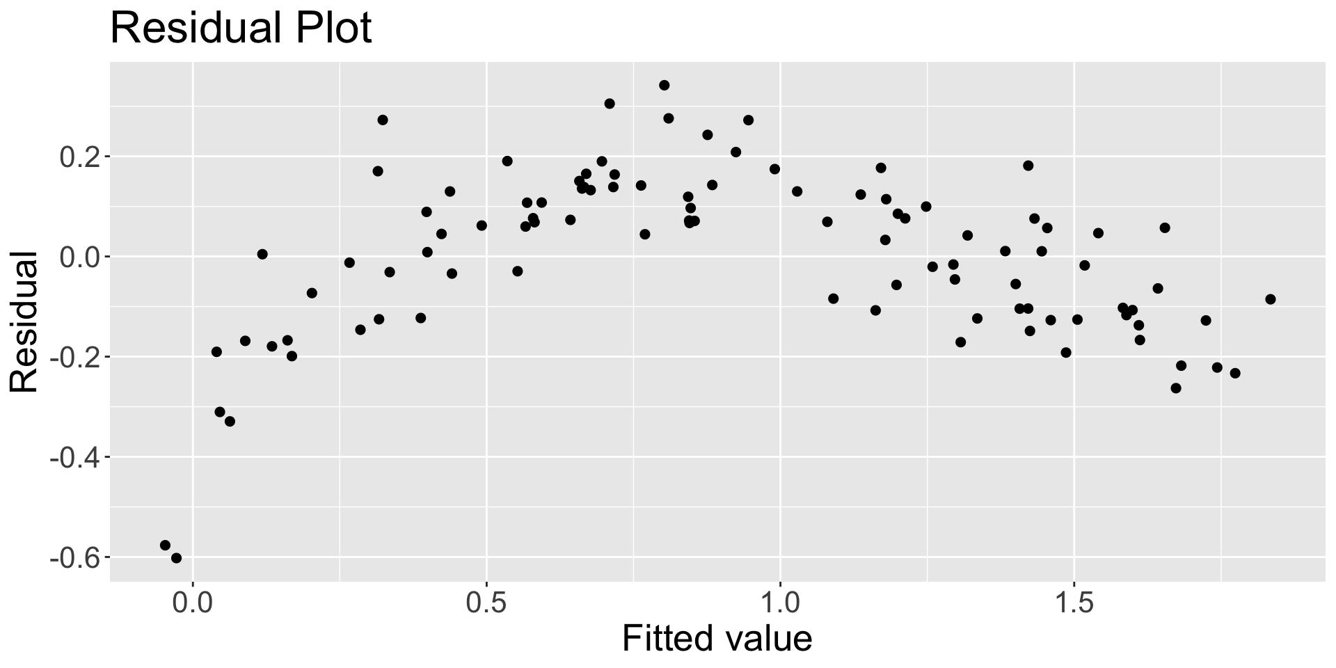
  • If the relationship between \(Y\) and \(x\) is not linear, then the residual-vs-fitted value plot may show a curved pattern.
  • One could argue that we could use the scatter plot of \(Y\) against \(x\) to detect nonlinearity.
    • However, the residual-vs-fitted value plot is often more effective because the scale of \(Y\) may obscure the nonlinearity.
    • Note how the residual plot clearly shows a curved pattern, while the scatter plot of \(Y\) against \(x\) is not as clear.
    • Besides, if we have more than one covariate, then the residual-vs-fitted value plot is easier to interpret.

Residuals vs fitted value: Heteroscedasticity

Scroll down

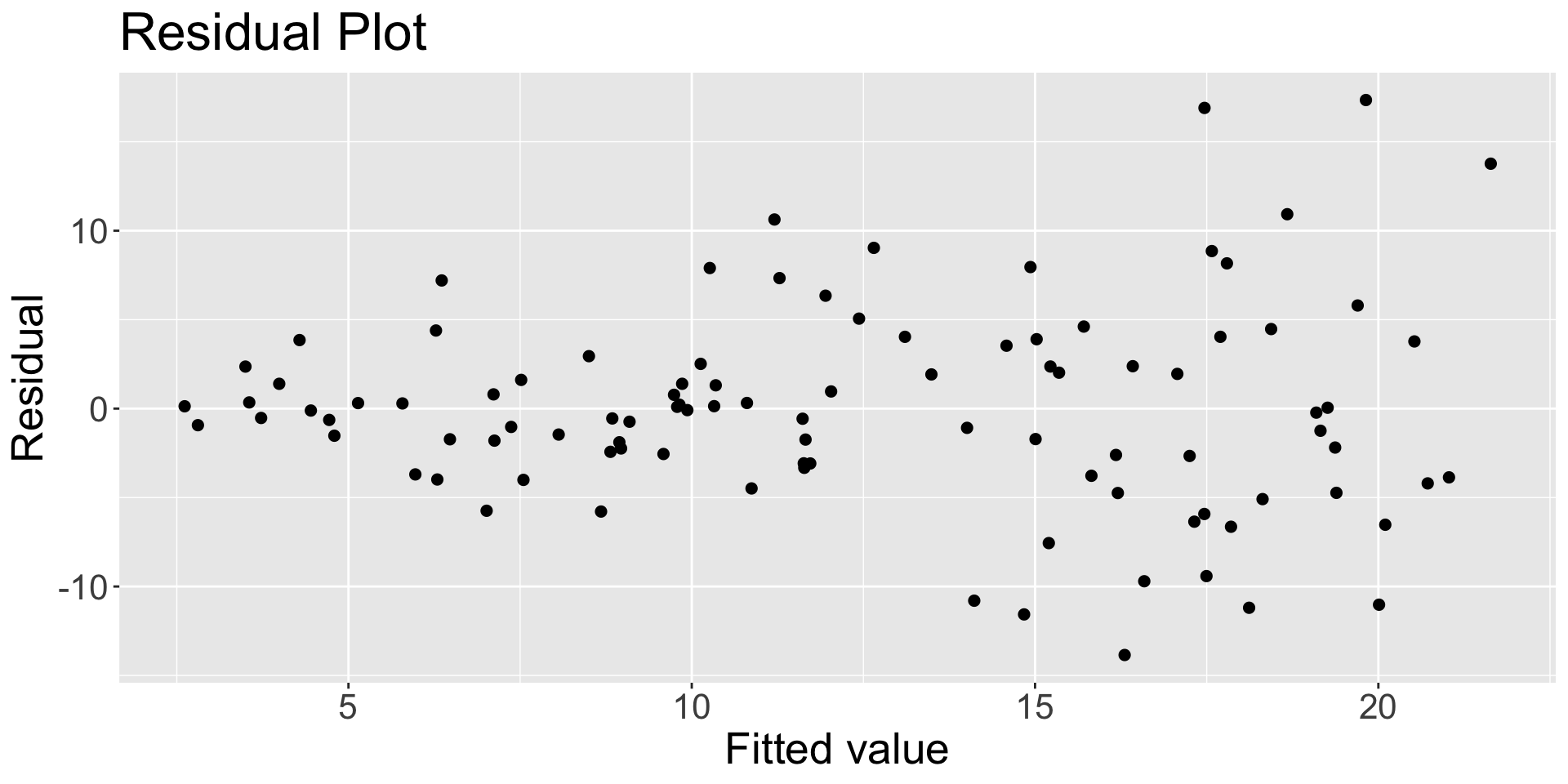
  • If the variance of the errors is not constant (i.e., the errors are heteroscedastic), then the residual-vs-fitted value plot may show a “fanning” pattern.
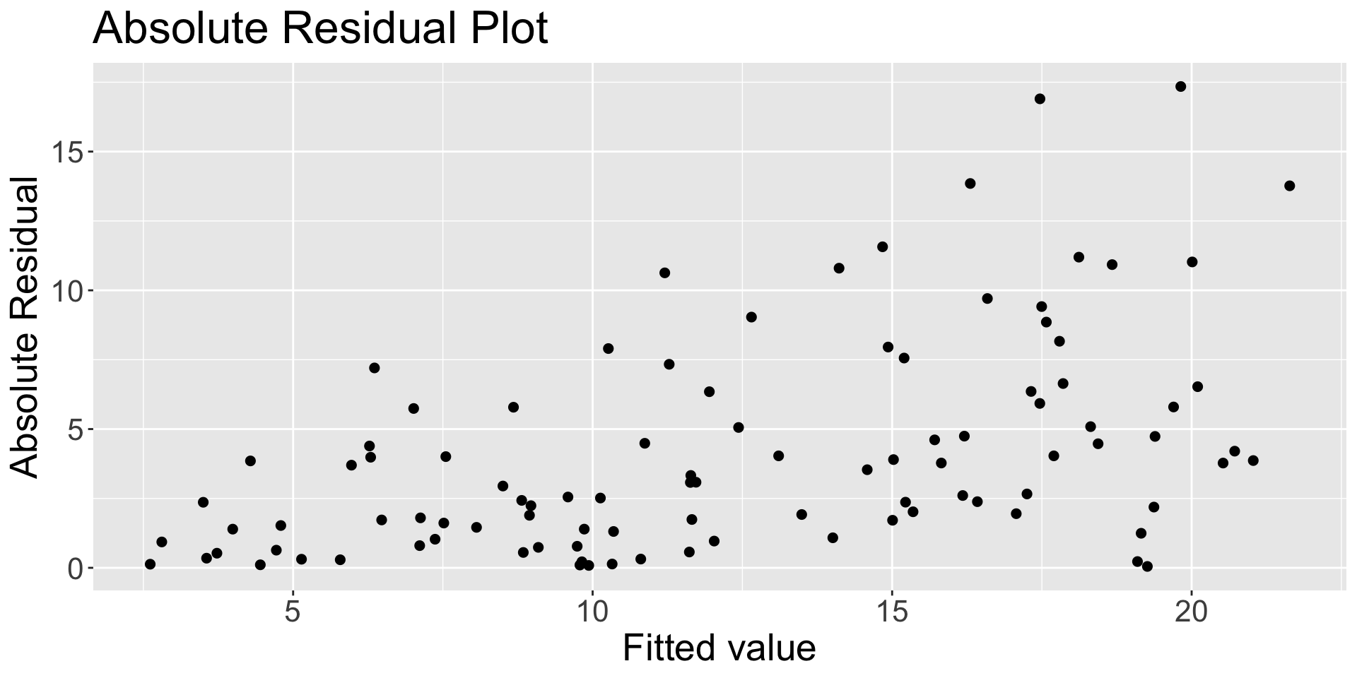
  • Another useful plot for detecting heteroscedasticity is the absolute residuals against the fitted value
QQ plot: Checking normality of residuals

Scroll down

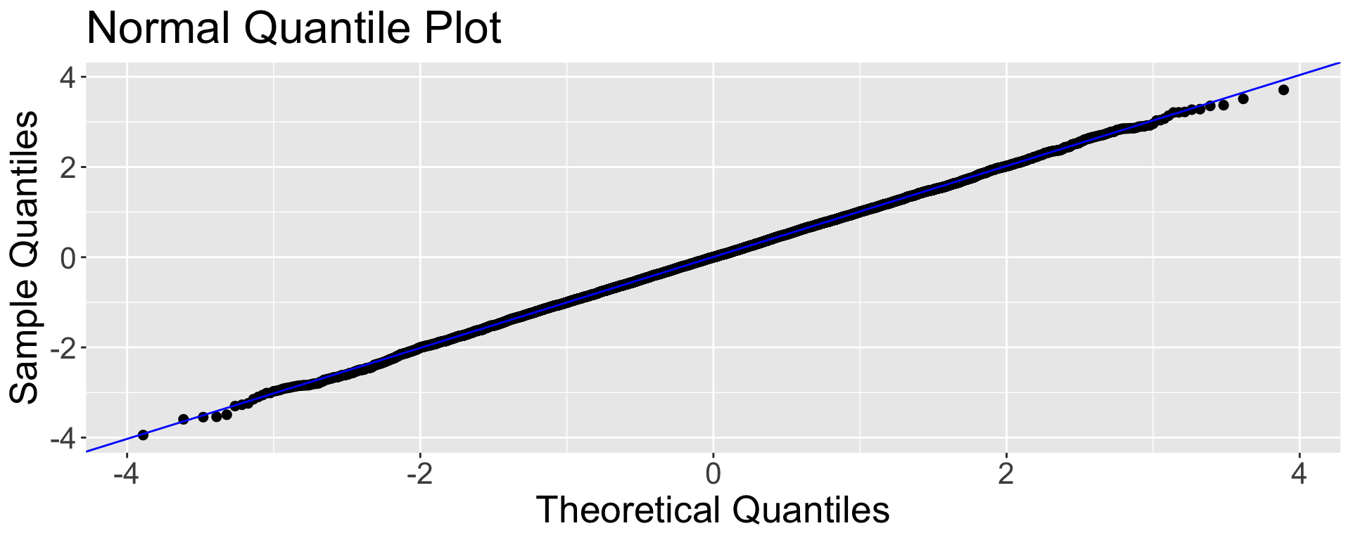
  • The normality assumption for the errors can be checked using a normal quantile plot of the residuals.

  • A normal quantile plot (sometimes called a normal probability plot) plots the ordered residuals \(e_{(1)}\leq\dotsc\leq e_{(n)}\) against \(\mathbb{E}[Z_{(1)}]\leq\dotsc\leq \mathbb{E}[Z_{(n)}]\), where \(Z_{(1)}\leq\dotsc\leq Z_{(n)}\) are an ordered sample of size \(n\) from \(N(0,1)\).

  • If the distribution of the residuals is close to normal, then the residual quantiles should resemble the expected quantiles, and so the points in the plot should lie closely along a straight line that has an intercept of \(0\) and a slope of \(\sigma\).
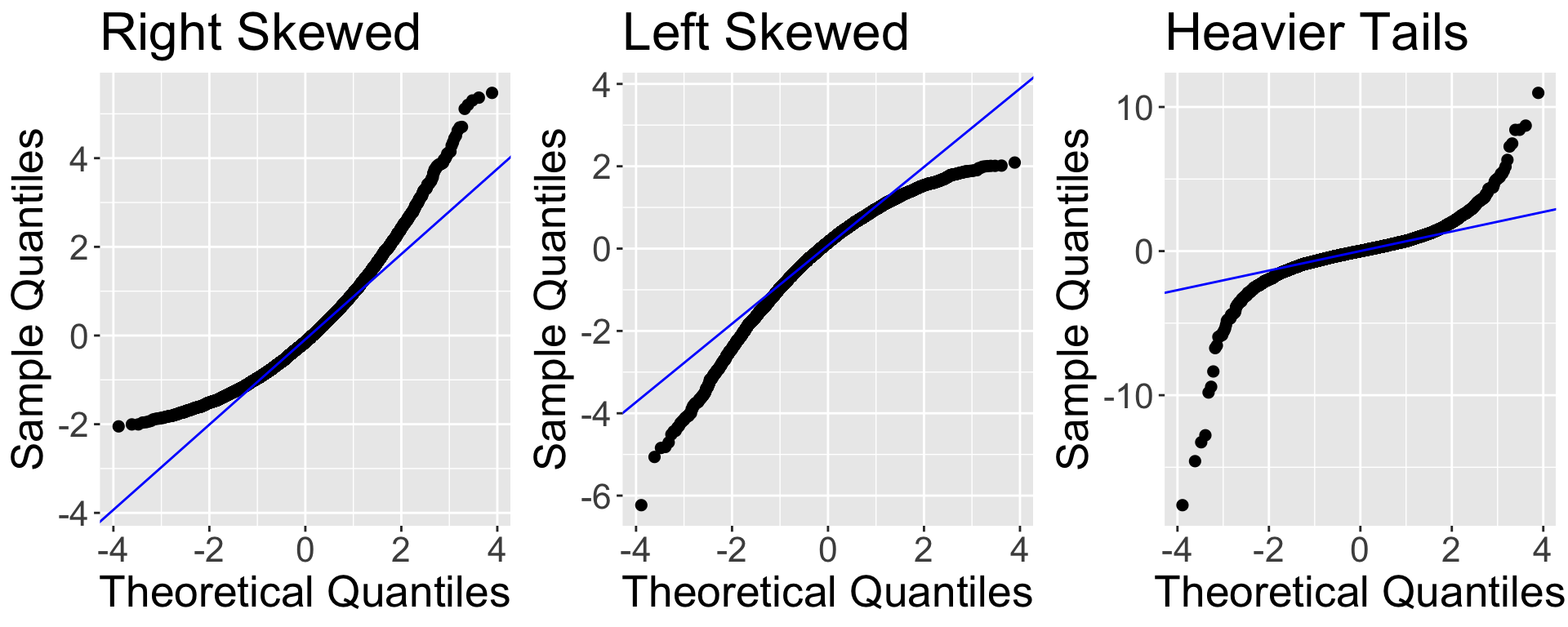
  • Small deviations from normality are not a big concern because the inference procedures (e.g., hypothesis tests and confidence intervals) based on the linear model are fairly robust to mild departures from normality, especially when the sample size is large.
    • Prediction intervals are more sensitive to non-normality.
  • Note that it is common to see some small deviations from normality in the tails of the normal quantile plot, even when the errors are normally distributed.
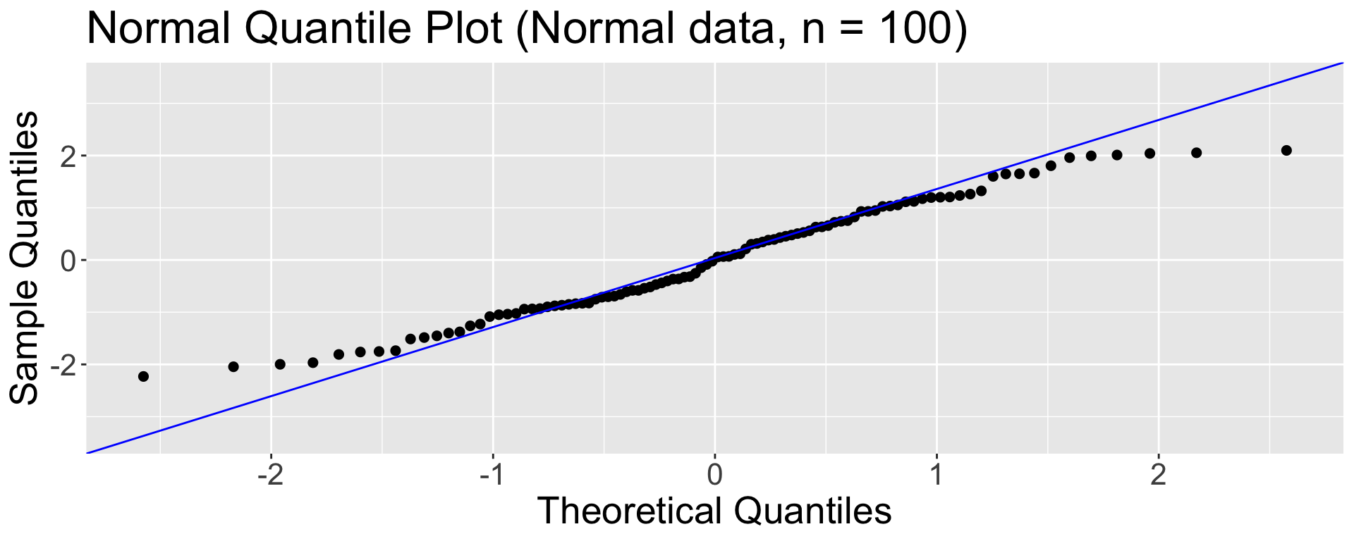
  • If you observe such deviations when your sample size is (very) large, then it may indicate that the errors are not normally distributed.

Serial correlation

  • When the covariate represents (most commonly) discrete time points, serial correlation (or more generally, autocorrelation) refers to the correlations in the responses across time points.

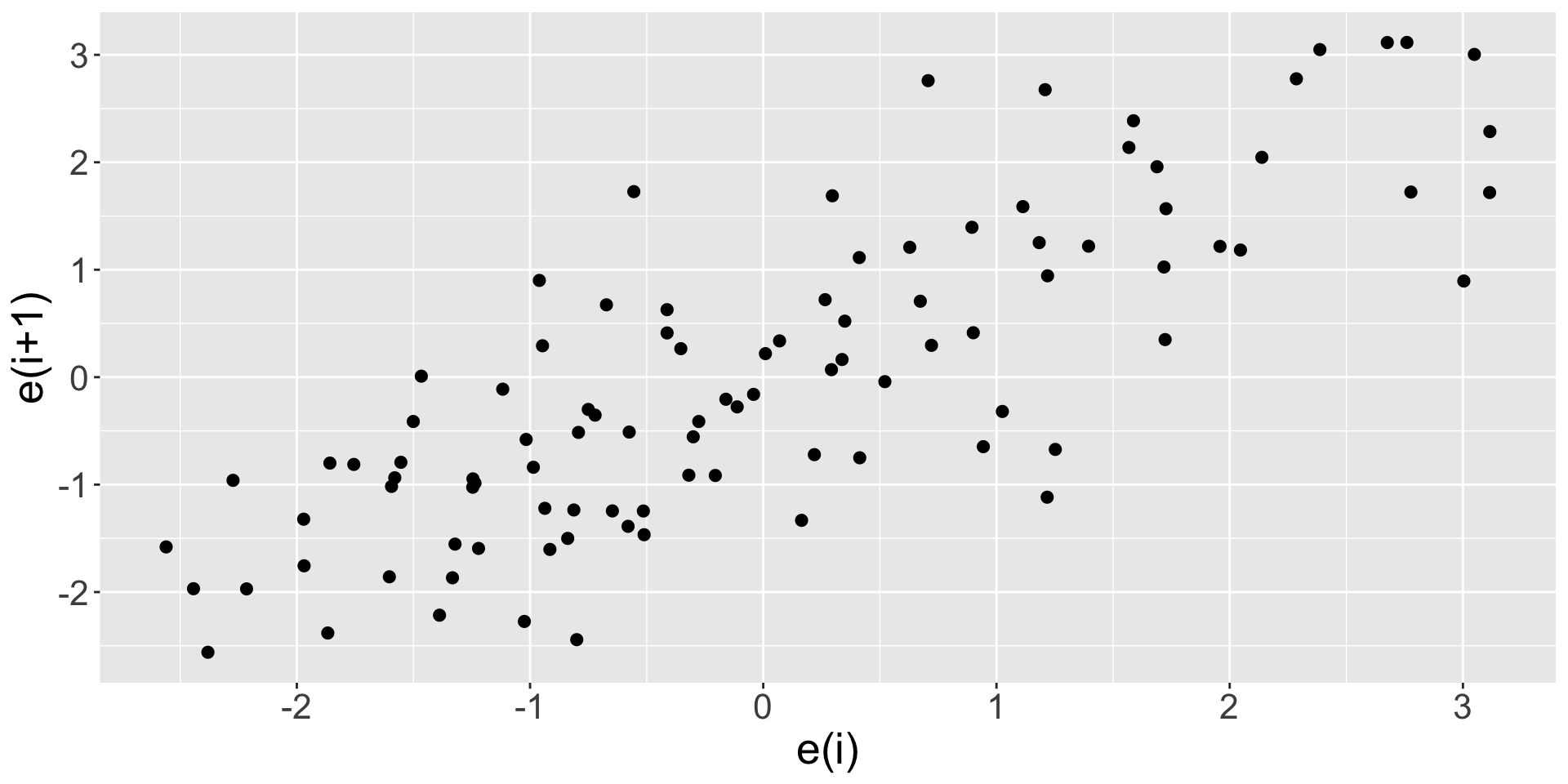
  • If there is no serial correlation, then plotting sequential residuals \(e_{i+1}\) against \(e_i\) should show no obvious patterns.

  • The following shows an example with serial correlation where the data are generated from an order-\(1\) autoregressive model \[ Y_i = Y_{i-1} + \varepsilon_i \;, \qquad Y_1 = \varepsilon_1 \;,\qquad \varepsilon_i\sim N(0,1) \;. \] (Note: models that account for autocorrelation, such as the autoregressive model, are outside the scope of STAT 306. Such models are the focus of STAT 443, which looks at time series data.)
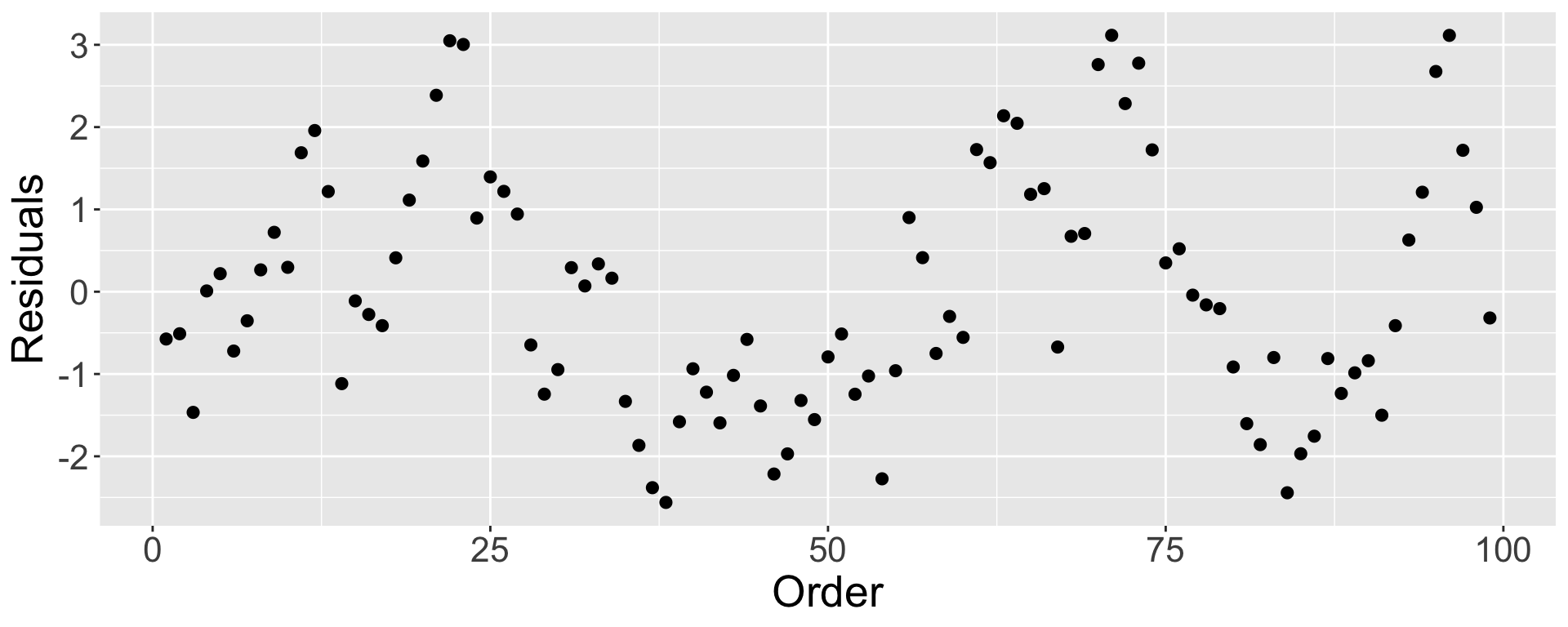
  • Another useful plot for detecting serial correlation is the plot of residuals against time (or order of observation).
Activity

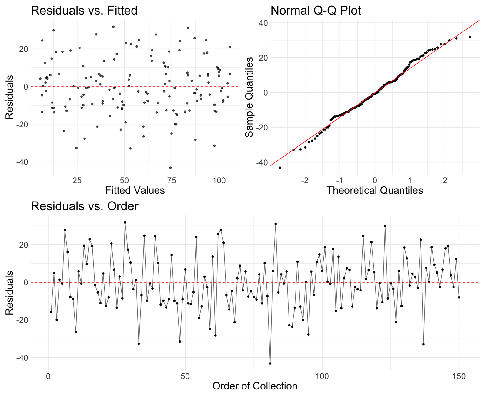
  • In R, you can plot a model object to get a series of diagnostic plots.
    • One of them is the leverage plot, which we will cover later in the course.
  • Time for iClickers!!

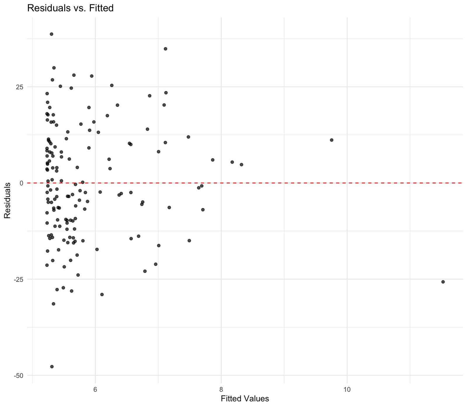
iClicker 1

Based on the diagnostic plots, which of the following is the primary conclusion about this regression model?


  1. The relationship is non-linear.
  2. The errors are not normally distributed.
  3. The variance of the errors is not constant (heteroscedasticity).
  4. There is strong evidence of serial correlation.
  5. There are no apparent major violations of the model assumptions.
iClicker 1: Solution

Based on the diagnostic plots, which of the following is the primary conclusion about this regression model?


  1. The relationship is non-linear.
  2. The errors are not normally distributed.
  3. The variance of the errors is not constant (heteroscedasticity).
  4. There is strong evidence of serial correlation.
  5. There are no apparent major violations of the model assumptions.
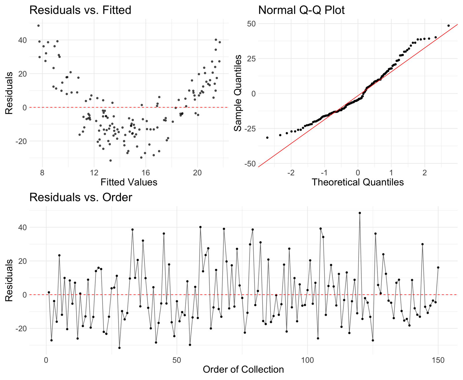
iClicker 2

Based on the diagnostic plots, which of the following is the primary conclusion about this regression model?


  1. The relationship is non-linear.
  2. The covariate is irrelevant.
  3. The variance of the errors is not constant (heteroscedasticity).
  4. There is strong evidence of serial correlation.
  5. There are no apparent major violations of the model assumptions.
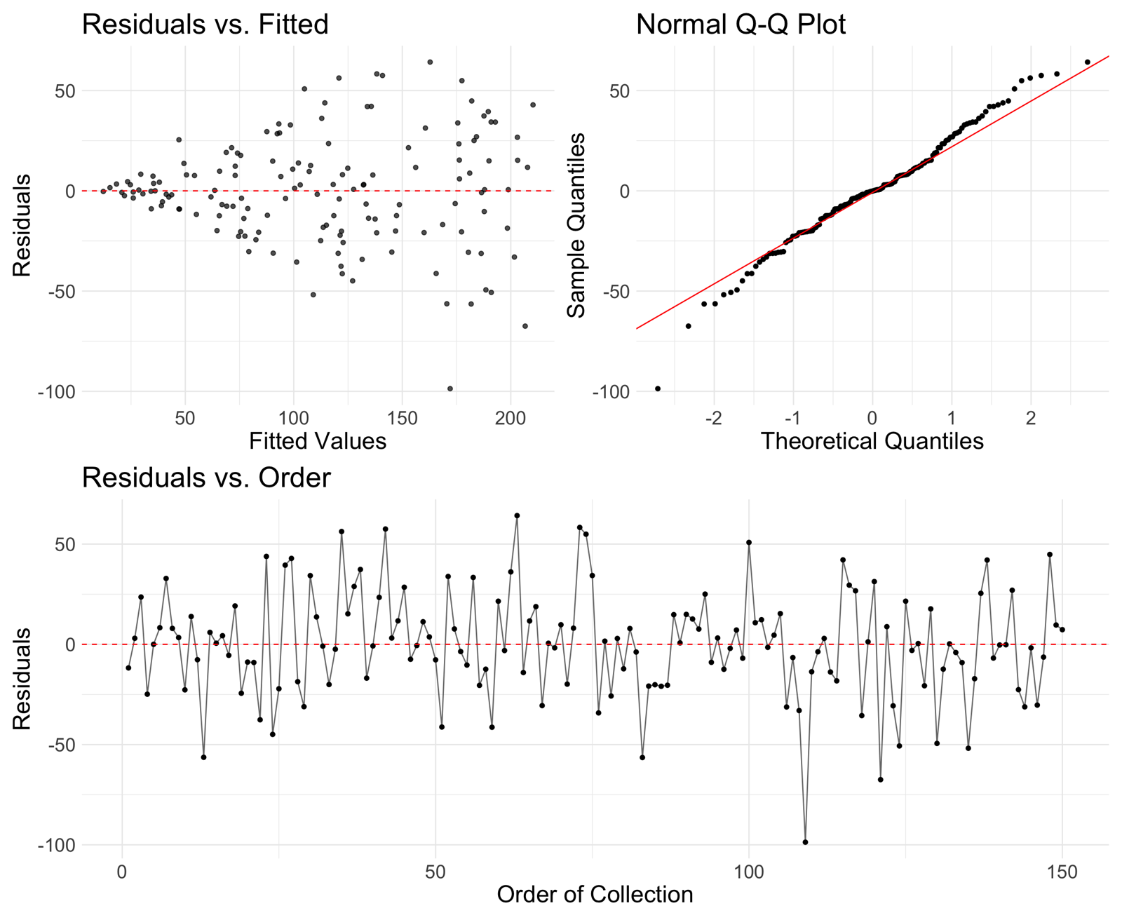
iClicker 2: Solution

Based on the diagnostic plots, which of the following is the primary conclusion about this regression model?


  1. The relationship is non-linear.
  2. The covariate is irrelevant.
  3. The variance of the errors is not constant (heteroscedasticity).
  4. There is strong evidence of serial correlation.
  5. There are no apparent major violations of the model assumptions.
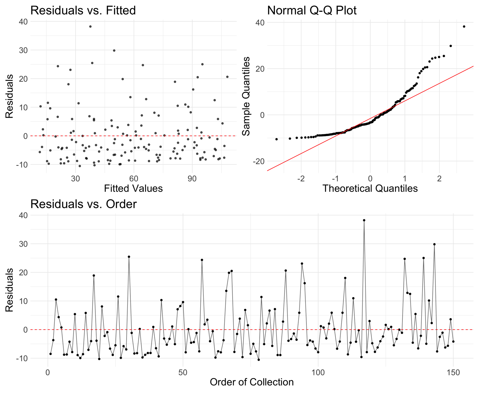
iClicker 3

Based on the diagnostic plots, which of the following is the primary conclusion about this regression model?


  1. The relationship is non-linear.
  2. The errors are not normally distributed.
  3. The variance of the errors is not constant (heteroscedasticity).
  4. There is strong evidence of serial correlation.
  5. There are no apparent major violations of the model assumptions.
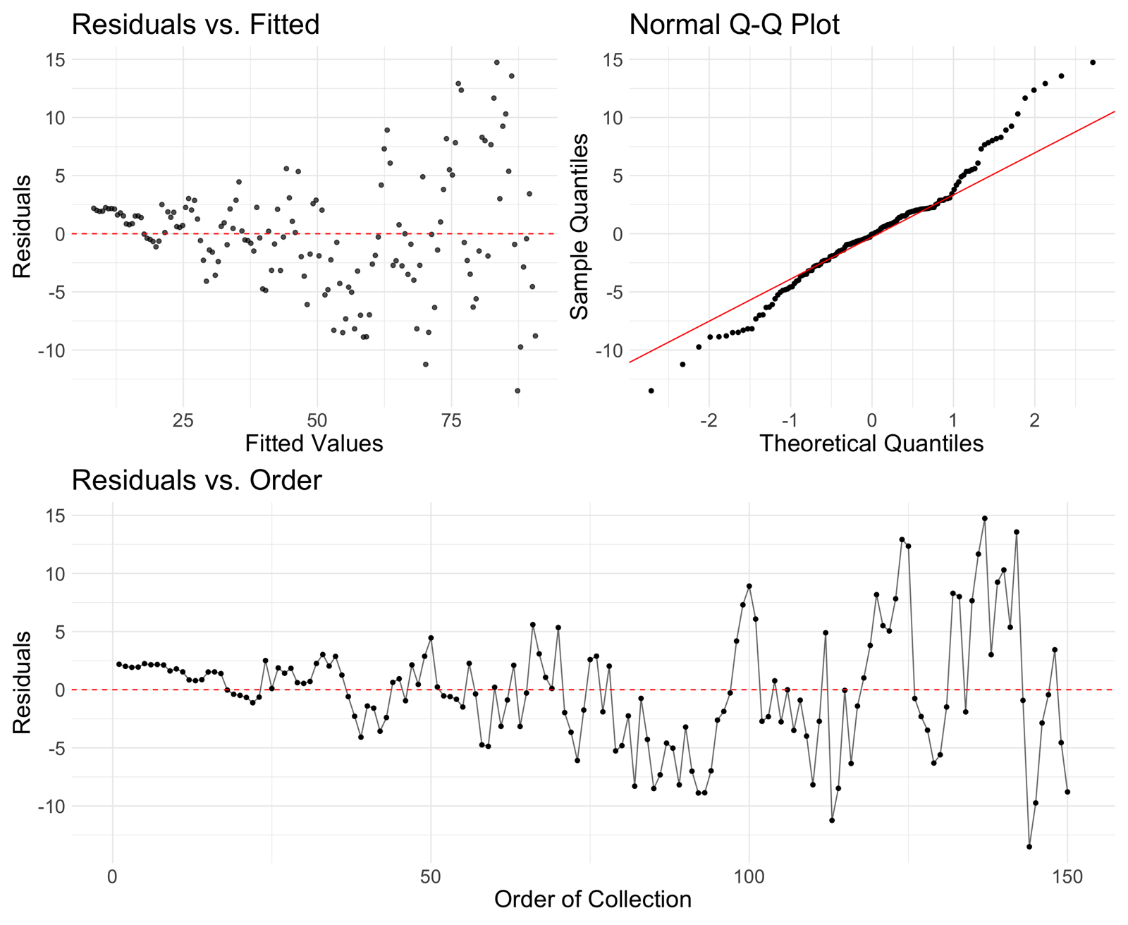
iClicker 3: Solution

Based on the diagnostic plots, which of the following is the primary conclusion about this regression model?


  1. The relationship is non-linear.
  2. The errors are not normally distributed.
  3. The variance of the errors is not constant (heteroscedasticity).
  4. There is strong evidence of serial correlation.
  5. There are no apparent major violations of the model assumptions.

iClicker 4

Based on the diagnostic plots, which of the following is the primary conclusion about this regression model?


  1. The relationship is non-linear.
  2. The errors are not normally distributed.
  3. The variance of the errors is not constant (heteroscedasticity).
  4. There is strong evidence of serial correlation.
  5. There are no apparent major violations of the model assumptions.

iClicker 4: Solution

Based on the diagnostic plots, which of the following is the primary conclusion about this regression model?


  1. The relationship is non-linear.
  2. The errors are not normally distributed.
  3. The variance of the errors is not constant (heteroscedasticity).
  4. There is strong evidence of serial correlation.
  5. There are no apparent major violations of the model assumptions.

iClicker 5

Based on the diagnostic plots, which of the following is the primary conclusion about this regression model?


  1. Non-linearity and non-normality.
  2. Non-linearity and serial correlation.
  3. Heteroscedasticity and serial correlation.
  4. Non-linearity and heteroscedasticity.
  5. There are no apparent major violations of the model assumptions.

iClicker 5: Solution

Based on the diagnostic plots, which of the following is the primary conclusion about this regression model?


  1. Non-linearity and non-normality.
  2. Non-linearity and serial correlation.
  3. Heteroscedasticity and serial correlation.
  4. Non-linearity and heteroscedasticity.
  5. There are no apparent major violations of the model assumptions.

iClicker 6

Based on the diagnostic plots, which of the following is the primary conclusion about this regression model?


  1. The relationship is non-linear.
  2. The errors are not normally distributed.
  3. The variance of the errors is not constant (heteroscedasticity).
  4. There is strong evidence of serial correlation.
  5. There are no apparent major violations of the model assumptions based on this plot alone.
iClicker 6: Solution

Based on the diagnostic plots, which of the following is the primary conclusion about this regression model?


  1. The relationship is non-linear.
  2. The errors are not normally distributed.
  3. The variance of the errors is not constant (heteroscedasticity).
  4. There is strong evidence of serial correlation.
  5. There are no apparent major violations of the model assumptions based on this plot alone.

Measure of linear association

Activity

  • Show that \[\sum_{i=1}^n (Y_i-\bar{Y})^2 = \sum_{i=1}^n (\hat{Y}_i - \bar{Y})^2 + \sum_{i=1}^n (Y_i-\hat{Y}_i)^2\]

  • What does each of the three terms represent?

Coefficient of determination: \(R^2\)

  • We have that:

\[ \begin{align} \sum_{i=1}^n (Y_i-\bar{Y})^2 &= \sum_{i=1}^n (Y_i-\hat{Y}_i + \hat{Y}_i - \bar{Y})^2\\ &= \sum_{i=1}^n (\hat{Y}_i - \bar{Y})^2 + \sum_{i=1}^n (Y_i-\hat{Y}_i)^2 + 2\sum_{i=1}^n (Y_i-\hat{Y}_i)(\hat{Y}_i - \bar{Y})\\ &= \sum_{i=1}^n (\hat{Y}_i - \bar{Y})^2 + \sum_{i=1}^n (Y_i-\hat{Y}_i)^2 \end{align} \]

  • Because, \[ \begin{align} \sum_{i=1}^n (Y_i-\hat{Y}_i)(\hat{Y}_i - \bar{Y}) &= \sum_{i=1}^n e_i(\hat{Y}_i - \bar{Y})\\ &= \hat{\beta}_0\sum_{i=1}^n e_i + \hat{\beta}_1\sum_{i=1}^n e_i x_i - \bar{Y}\sum_{i=1}^n e_i\\ &= 0 + 0 - 0\\ &= 0 \end{align} \]

Coefficient of determination: \(R^2\)

  • Note that \(\sum_{i=1}^n (Y_i-\bar{Y})^2\) measures the total variability in the response \(Y\), and is called total sum of squares (TSS).
  • The term \(\sum_{i=1}^n (\hat{Y}_i - \bar{Y})^2\) measures the variability in the fitted values \(\hat{Y}_i\), and is called model sum of squares (MSS).
    • Usually, this term is referred to as regression sum of squares (RSS) in the context of regression analysis. But this will be confusing with the residual sum of squares (RSS).
  • The term \(\sum_{i=1}^n (Y_i-\hat{Y}_i)^2\) measures the variability in the residuals \(e_i\), and is called residual sum of squares (RSS).
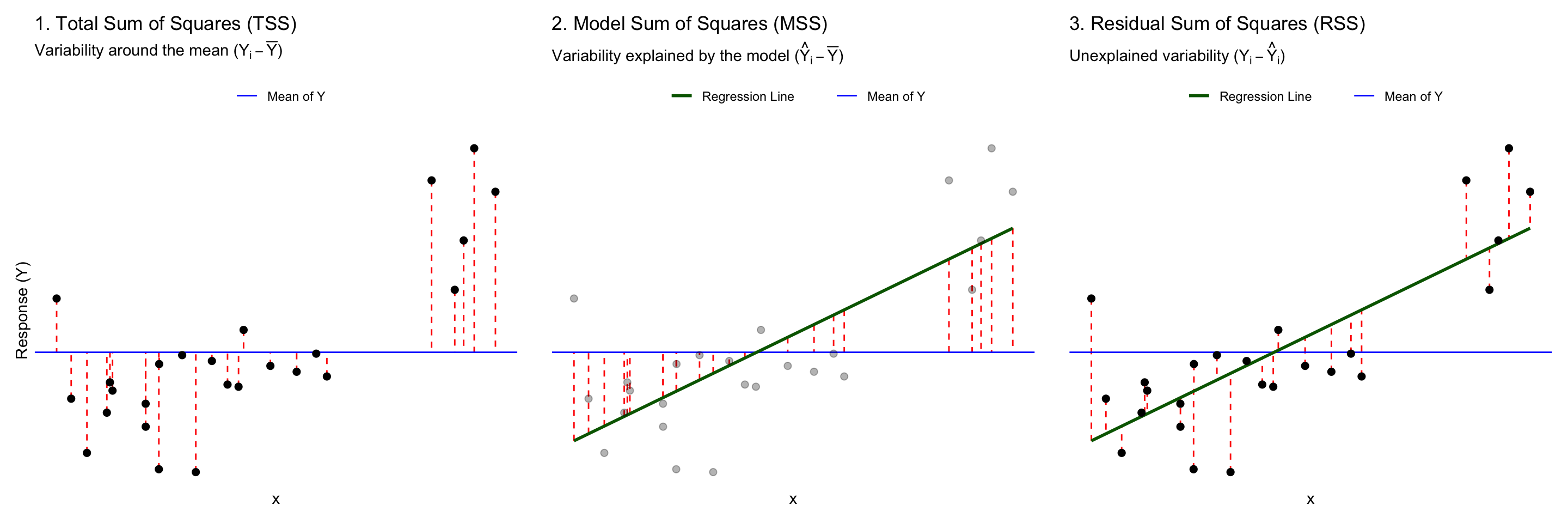
Figure 1: Visual decomposition of the Total Sum of Squares (TSS) into Model (MSS) and Residual (RSS) components.

Coefficient of determination: \(R^2\)

  • From \(\sum_{i=1}^n (Y_i-\bar{Y})^2 = \sum_{i=1}^n (\hat{Y}_i - \bar{Y})^2 + \sum_{i=1}^n (Y_i-\hat{Y}_i)^2\), we can write \[ \begin{align} TSS &= MSS + RSS \\ 1 &= \frac{MSS}{TSS} + \frac{RSS}{TSS} \end{align} \]
  • The term \(R^2 = \frac{MSS}{TSS} = 1 - \frac{RSS}{TSS}\) is called the coefficient of determination.
    • \(R^2\) measures the proportion of variability in the response \(Y\) that is explained by the linear model.
    • This decomposition is reliant on the use of the least squares method to fit the linear model.
    • It takes values between \(0\) and \(1\).
    • A value close to \(1\) indicates that a large proportion of the variability in \(Y\) is explained by the model, while a value close to \(0\) indicates that the model explains very little of the variability in \(Y\).
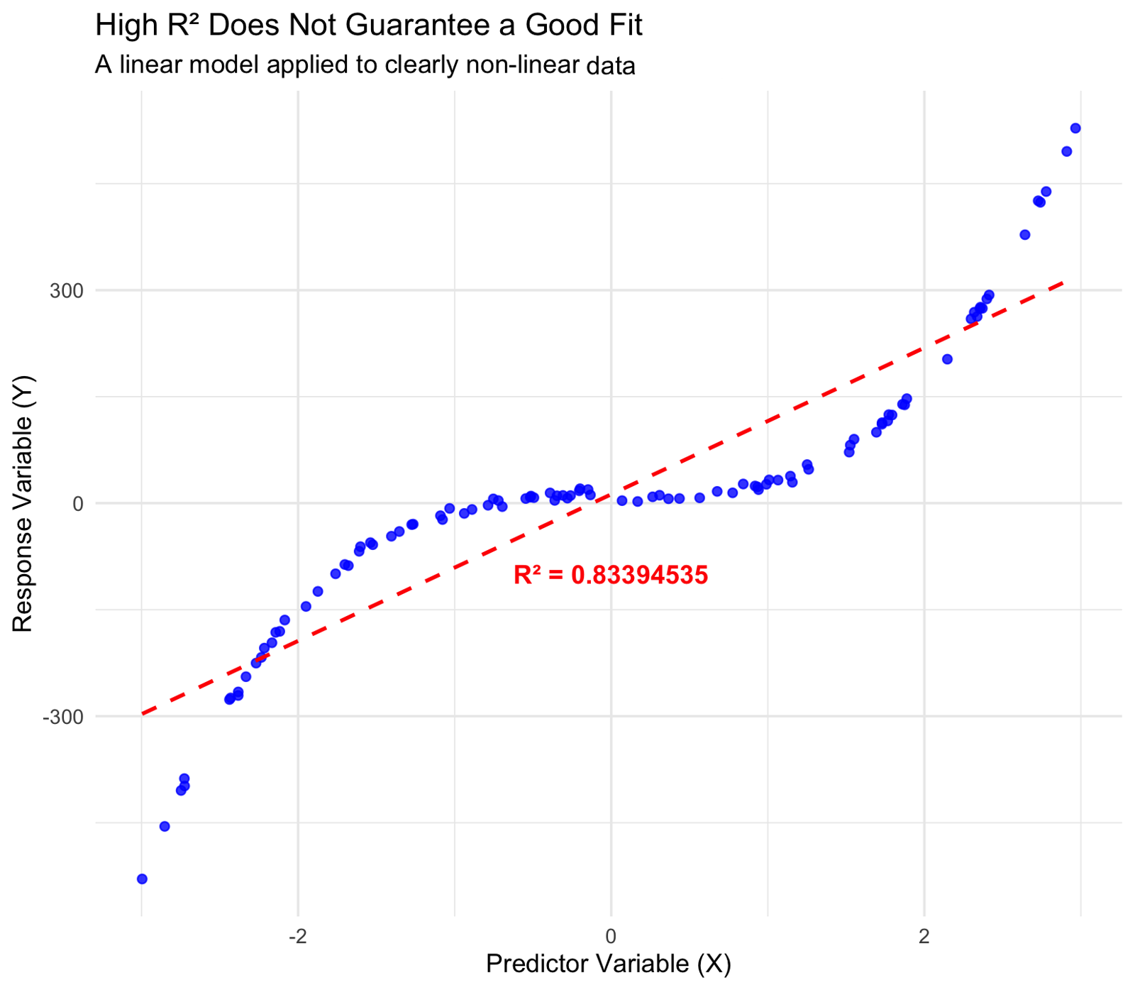
    • Note that a high value of \(R^2\) does not necessarily mean that the model is appropriate for the data.
      • Always check the model assumptions using residual plots.

iClicker 7

True or False: A high \(R^2\) means our model is a good fit.

  1. True.
  2. False.

iClicker 7: Solution

True or False: A high \(R^2\) means our model is a good fit.

  1. True.
  2. False.

iClicker 8

True or False: A high \(R^2\) means that our predictions will be accurate.

  1. True.
  2. False.

iClicker 8: Solution

True or False: A high \(R^2\) means that our predictions will be accurate.

  1. True.
  2. False.

iClicker 9

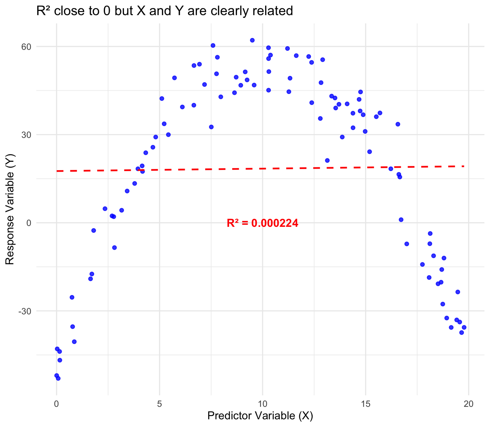
True or False: A \(R^2 \approx 0\) means \(X\) and \(Y\) are not related.

  1. True.
  2. False.

iClicker 9: Solution

True or False: A \(R^2 \approx 0\) means \(X\) and \(Y\) are not related.

  1. True.
  2. False.

Post-Lecture Exercise

  • Show that in simple linear regression, \(R^2\) is the square of the correlation coefficient between \(X\) and \(Y\).

Solution:

We want to prove that \(R^2 = r^2\). We start with the definition \(R^2 = \frac{MSS}{TSS}\). Let \(S_{xx} = \sum (x_i - \bar{x})^2\), \(S_{yy} = \sum (y_i - \bar{y})^2\), and \(S_{xy} = \sum (x_i - \bar{x})(y_i - \bar{y})\). Then,

\[ \begin{align*} R^2 &= \frac{MSS}{TSS} \\ &= \frac{\sum(\hat{y}_i - \bar{y})^2}{S_{yy}} \\ &= \frac{\sum(\bar{y}+\hat{\beta}_1(x_i - \bar{x})-\bar{y})^2}{S_{yy}} \\ &= \frac{\sum(\hat{\beta}_1(x_i - \bar{x}))^2}{S_{yy}} \\ &= \frac{\hat{\beta}_1^2 \sum(x_i - \bar{x})^2}{S_{yy}} \\ &= \frac{\hat{\beta}_1^2 S_{xx}}{S_{yy}} \\ &= \frac{(S_{xy}/S_{xx})^2 S_{xx}}{S_{yy}} \\ &= \frac{S_{xy}^2}{S_{xx}S_{yy}} \\ &= \left(\frac{S_{xy}}{\sqrt{S_{xx}S_{yy}}}\right)^2 \\ &= r^2 \end{align*} \]

Simpson’s Paradox

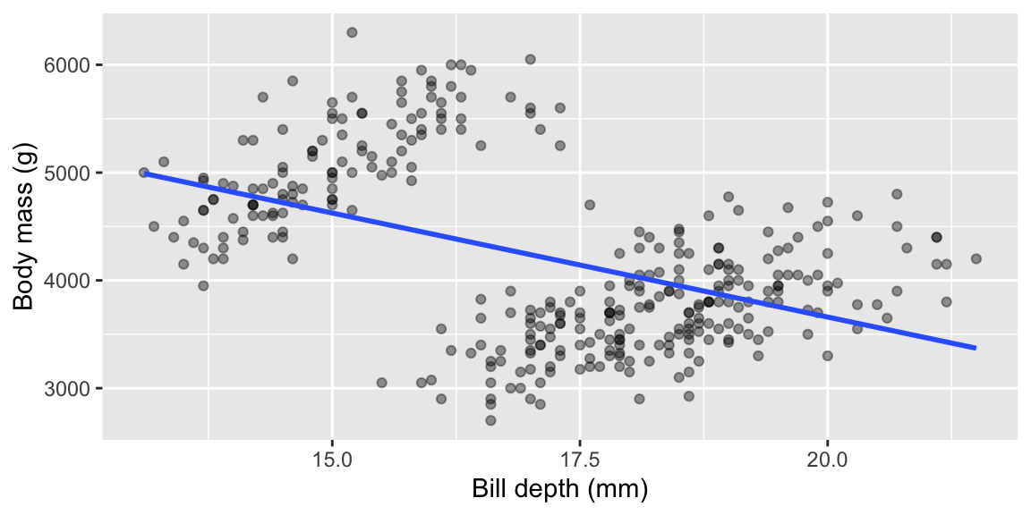
  • Let’s fit a model to explain penguins’ body mass based on the bill depth.

  • This model suggests that an increase in the bill depth is associated with a decrease in body mass!

Call:
lm(formula = body_mass_g ~ bill_depth_mm, data = penguins_clean)

Coefficients:
  (Intercept)  bill_depth_mm  
         7520           -193  

Simpson’s Paradox

  • But if we fit one linear regression per species, we get…
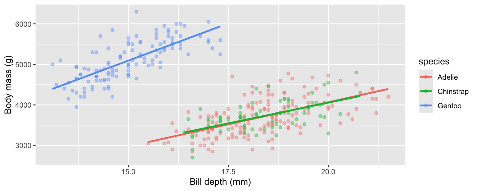
  • By controlling for species, the correlation between bill depth and body mass becomes positive.

About linearity

  • We keep saying that we assume a linear relationship between \(X\) and \(Y\).

    • But what does that really mean?
  • The linearity assumption is linear in the parameters. For example:

    • The model \(Y = \beta_0 + \beta_1 X^2 + \varepsilon\) is still a linear model, even though it includes a quadratic term in \(X\).
    • The model \(Y = \beta_0 + \beta_1 \log(X) + \varepsilon\) is also a linear model, even though it includes a logarithmic transformation of \(X\).
    • The model \(Y = \beta_0 + \beta_1 e^X + \varepsilon\) is also a linear model, even though it includes an exponential transformation of \(X\).
  • We can just think of \(Z = X\), \(Z = X^2\), \(Z = \log(X)\), \(Z = e^X\), etc., and then fit a linear model of the form \[ Y_i = \beta_0 + \beta_1 Z_i + \varepsilon_i \]

  • The model is not linear if it includes terms like \(\sin(\beta_1 X)\).

    • Think about the derivation of the least squares estimates in this case.

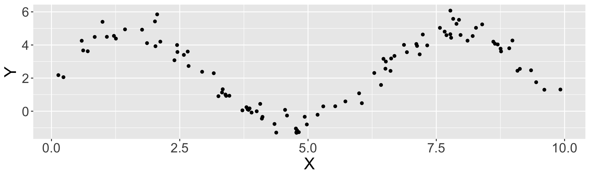
Linearity: Example

  • Suppose we have the following data:

  • If we fit a linear model of the form \(Y_i = \beta_0 + \beta_1 \sin(x_i) + \varepsilon_i\), we get:
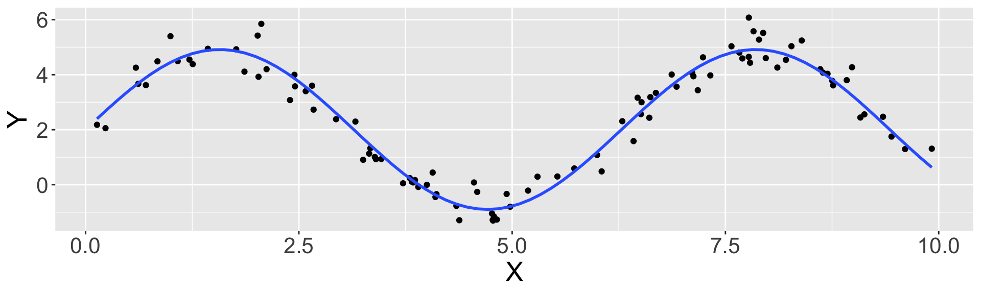
  • Everything we discussed is valid for this model as well.

What We Learned

  • Residual Diagnostics: We cannot observe the errors \(\varepsilon_i\), so we use the residuals \(e_i\) as a proxy to check the model assumptions.

    • Least squares forces \(\sum_{i=1}^n e_i = 0\) and \(\sum_{i=1}^n x_i e_i = 0\), so the mean of the residuals tells us nothing about \(\mathbb{E}[\varepsilon_i] = 0\).
  • What to Look for in the Plots:

    • Residuals vs. fitted values (or \(x\)): should show no pattern. A curve suggests non-linearity; a fan shape suggests heteroscedasticity.
    • Normal quantile plot: points should lie close to a straight line. Skewness and heavy tails show up as systematic departures; small departures in the tails are common, especially for small \(n\).
    • \(e_{i+1}\) vs. \(e_i\) and residuals vs. order: should show no pattern. A pattern suggests serial correlation.
  • Sum of Squares Decomposition: For least squares with an intercept, \[ \underbrace{\sum_{i=1}^n (Y_i-\bar{Y})^2}_{TSS} = \underbrace{\sum_{i=1}^n (\hat{Y}_i - \bar{Y})^2}_{MSS} + \underbrace{\sum_{i=1}^n (Y_i-\hat{Y}_i)^2}_{RSS} \]

  • Coefficient of Determination: \(R^2 = \dfrac{MSS}{TSS} = 1 - \dfrac{RSS}{TSS}\) is the proportion of the variability in \(Y\) explained by the linear model.

    • In simple linear regression, \(R^2 = r^2\), the squared correlation between \(X\) and \(Y\).
    • A high \(R^2\) does not imply a good fit or accurate predictions, and \(R^2 \approx 0\) does not imply that \(X\) and \(Y\) are unrelated.
  • Linearity and Simpson’s Paradox:

    • “Linear” means linear in the parameters, so transformations such as \(X^2\), \(\log(X)\), or \(\sin(X)\) can be used as the covariate; \(\sin(\beta_1 X)\) cannot.
      • But note that the interpretation of \(\beta_1\) now is about the expected change in \(Y\) for a one-unit increase in the transformed variable (e.g., \(\sin(X)\)), not \(X\), which is not as straightforward as before.
    • Ignoring a relevant variable (e.g., species) can reverse the direction of an association.