Inference for Least Squares Estimators
STAT 306 - Module 04
Learning Objectives
- By the end of this lecture, you should be able to:
- Estimate the error variance \(\sigma^2\) using the residual variance \(s^2\).
- Compute the estimated standard errors \(\widehat{\text{SE}}(\widehat{\beta}_0)\) and \(\widehat{\text{SE}}(\widehat{\beta}_1)\).
- State the \(t\)-distribution of standardized regression estimators with \(n-2\) degrees of freedom.
- Construct and interpret confidence intervals for \(\beta_0\) and \(\beta_1\).
- Conduct hypothesis tests for regression parameters and interpret \(p\)-values.
Simple Linear Regression: Review
- Given data \((x_i,y_i)\), \(i=1,\dotsc,n\), we consider a linear model of the form \[ Y_i = \beta_0 + \beta_1x_i + \varepsilon_i \;, \qquad \varepsilon_i \overset{\text{iid}}{\sim} N(0,\sigma^2) \;, \] where \(\beta_0\) and \(\beta_1\) are unknown parameters and \(x_1,\dotsc,x_n\) are treated as fixed constants.
- Fitting the linear model means finding values of the intercept \(b_0\) and slope \(b_1\) that minimize the Residual Sum of Squares: \[ RSS(b_0,b_1) = \sum_{i=1}^n e_i^2 = \sum_{i=1}^n \left[y_i - (b_0 + b_1 x_i)\right]^2 \;. \]
- The solution to this optimization problem gives the least squares estimators:
\[ \begin{align} \widehat\beta_1 &= r_{XY}\frac{S_Y}{S_X} = \frac{\sum_{i=1}^n(x_i-\bar{x})(Y_i-\bar{Y})}{\sum_{i=1}^n(x_i-\bar{x})^2} = \frac{\sum_{i=1}^nx_iY_i - n\bar{x}\bar{Y}}{\sum_{i=1}^nx_i^2-n\bar{x}^2} \;, \\ \widehat\beta_0 &= \bar{Y} - \widehat\beta_1\bar{x} \; \end{align} \]
Sampling distributions of LSE
In Module 03, we derived the sampling distributions of the least squares estimators (LSE) \(\widehat{\beta}_0\) and \(\widehat{\beta}_1\).
We found that:
\[ \begin{align} \widehat{\beta}_1 \sim N\left(\beta_1, \frac{\sigma^2}{\sum_{i=1}^n(x_i-\bar{x})^2}\right) & \qquad \widehat{\beta}_0 \sim N\left(\beta_0, \sigma^2\left(\frac{1}{n} + \frac{\bar{x}^2}{\sum_{i=1}^n(x_i-\bar{x})^2}\right)\right) \; \end{align} \]
- Today, we will use these results for inference about the parameters \(\beta_0\) and \(\beta_1\).
Review of Confidence Intervals and Hypothesis Testing
iClicker 1
When we want to write \((1-\alpha)\times 100\%\) confidence intervals for a parameter \(\theta\), which of the following is the generic form?
- \(\hat{\theta} \pm c^*_{1-\frac{\alpha}{2}}\times \frac{\widehat{\text{SE}}(\hat{\theta})}{n}\)
- \(\hat{\theta} \pm c^*_{1-\frac{\alpha}{2}}\times \frac{\widehat{\text{SE}}(\hat{\theta})}{\sqrt{n}}\)
- \(\hat{\theta} \pm c^*_{1-\frac{\alpha}{2}}\times \frac{\text{SE}(\hat{\theta})}{\sqrt{n}}\)
- \(\hat{\theta} \pm c^*_{1-\frac{\alpha}{2}}\times \widehat{\text{SE}}(\hat{\theta})\)
- \(\hat{\theta} \pm c^*_{1-\frac{\alpha}{2}}\times \widehat{\text{Var}}(\hat{\theta})\)
iClicker 1: Solution
When we want to write \((1-\alpha)\times 100\%\) confidence intervals for a parameter \(\theta\), which of the following is the generic form?
- \(\hat{\theta} \pm c^*_{1-\frac{\alpha}{2}}\times \frac{\widehat{\text{SE}}(\hat{\theta})}{n}\)
- \(\hat{\theta} \pm c^*_{1-\frac{\alpha}{2}}\times \frac{\widehat{\text{SE}}(\hat{\theta})}{\sqrt{n}}\)
- \(\hat{\theta} \pm c^*_{1-\frac{\alpha}{2}}\times \frac{\text{SE}(\hat{\theta})}{\sqrt{n}}\)
- \(\hat{\theta} \pm c^*_{1-\frac{\alpha}{2}}\times \widehat{\text{SE}}(\hat{\theta})\)
- \(\hat{\theta} \pm c^*_{1-\frac{\alpha}{2}}\times \widehat{\text{Var}}(\hat{\theta})\)
iClicker 2
How does the width of a 95% confidence interval change as the sample size \(n\) increases?
- No change.
- The width decreases.
- The width increases.
- Not enough information.
iClicker 2: Solution
How does the width of a 95% confidence interval change as the sample size \(n\) increases?
- No change.
- The width decreases.
- The width increases.
- Not enough information.
Context
A group of educational researchers wants to estimate the average number of hours per week that full-time university students in a large state spend on academic activities outside of class time.
They randomly sample 200 full-time students from universities across the state. The sample mean is calculated to be 18.5 hours.
Then, a 95% confidence interval for the true mean number of hours spent on academic activities by all full-time university students in the state is calculated to be \([17.64, 19.36]\) hours.
iClicker 3
Is the following interpretation about this interval correct or incorrect?
There is a 95% probability that the true average number of hours spent on academic activities by all full-time university students in the state falls between 17.64 and 19.36 hours.
- Correct.
- Incorrect.
iClicker 3: Solution
Is the following interpretation about this interval correct or incorrect?
There is a 95% probability that the true average number of hours spent on academic activities by all full-time university students in the state falls between 17.64 and 19.36 hours.
- Correct.
- Incorrect.
iClicker 4
Is the following interpretation about this interval correct or incorrect?
If we were to repeat this sampling process many times, taking random samples of 200 students and calculating a 95% confidence interval for each sample, we would expect about 95% of those calculated intervals to contain the true average number of hours spent on academic activities by all full-time university students in the state.
- Correct.
- Incorrect.
iClicker 4: Solution
Is the following interpretation about this interval correct or incorrect?
If we were to repeat this sampling process many times, taking random samples of 200 students and calculating a 95% confidence interval for each sample, we would expect about 95% of those calculated intervals to contain the true average number of hours spent on academic activities by all full-time university students in the state.
- Correct.
- Incorrect.
iClicker 5
Is the following interpretation about this interval correct or incorrect?
We are 95% confident that the sample mean number of hours is between 17.64 and 19.36 hours.
- Correct.
- Incorrect.
iClicker 5: Solution
Is the following interpretation about this interval correct or incorrect?
We are 95% confident that the sample mean number of hours is between 17.64 and 19.36 hours.
- Correct.
- Incorrect.
iClicker 6
Is the following interpretation about this interval correct or incorrect?
95% of the full-time university students in the state spend between 17.64 and 19.36 hours per week on academic activities.
- Correct.
- Incorrect.
iClicker 6: Solution
Is the following interpretation about this interval correct or incorrect?
95% of the full-time university students in the state spend between 17.64 and 19.36 hours per week on academic activities.
- Correct.
- Incorrect.
iClicker 7
Is the following interpretation about this interval correct or incorrect?
We can be 95% confident that a randomly selected full-time university student from the state spends between 17.64 and 19.36 hours per week on academic activities.
- Correct.
- Incorrect.
iClicker 7: Solution
Is the following interpretation about this interval correct or incorrect?
We can be 95% confident that a randomly selected full-time university student from the state spends between 17.64 and 19.36 hours per week on academic activities.
- Correct.
- Incorrect.
iClicker 8
Is the following interpretation about this interval correct or incorrect?
Approximately 95% of the possible samples of size \(n\) we could select would give us a 95% confidence interval that captures the true average number of hours spent on academic activities by all full-time university students in the state.
- Correct.
- Incorrect.
iClicker 8: Solution
Is the following interpretation about this interval correct or incorrect?
Approximately 95% of the possible samples of size \(n\) we could select would give us a 95% confidence interval that captures the true average number of hours spent on academic activities by all full-time university students in the state.
- Correct.
- Incorrect.
iClicker 9
Suppose we want to test \(H_0: \mu = \mu_0\) vs \(H_A: \mu \neq \mu_0\). And our test statistic is \(T = 1\). Which panel below shows the correct p-value?
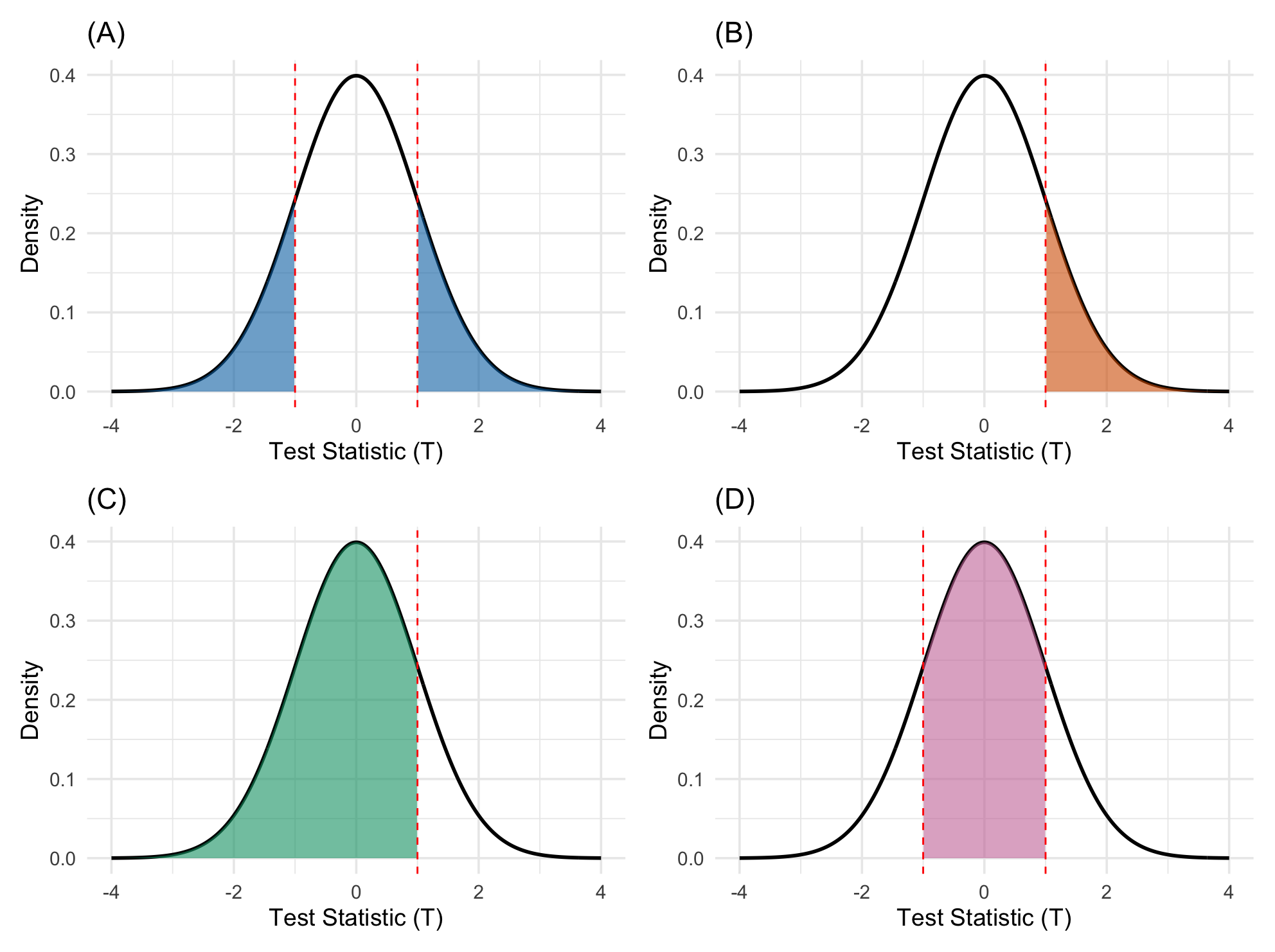
iClicker 9: Solution
Suppose we want to test \(H_0: \mu = \mu_0\) vs \(H_A: \mu \neq \mu_0\). And our test statistic is \(T = 1\). Which panel below shows the correct p-value?
Correct answer: Panel (A)
iClicker 10
Suppose we want to test \(H_0: \mu = \mu_0\) vs \(H_A: \mu < \mu_0\). And our test statistic is \(T = 1\). Which panel below shows the correct p-value?
iClicker 10: Solution
Suppose we want to test \(H_0: \mu = \mu_0\) vs \(H_A: \mu < \mu_0\). And our test statistic is \(T = 1\). Which panel below shows the correct p-value?
Correct answer: Panel (C)
iClicker 11
Suppose we want to test \(H_0: \mu = \mu_0\) vs \(H_A: \mu > \mu_0\). And our test statistic is \(T = 1\). Which panel below shows the correct p-value?
iClicker 11: Solution
Suppose we want to test \(H_0: \mu = \mu_0\) vs \(H_A: \mu > \mu_0\). And our test statistic is \(T = 1\). Which panel below shows the correct p-value?
Correct answer: Panel (B)
iClicker 12
Is the following statement true or false?
The null model is the sampling distribution of the test statistic when the null hypothesis is true.
- True.
- False.
iClicker 12: Solution
Is the following statement true or false?
The null model is the sampling distribution of the test statistic when the null hypothesis is true.
- True.
- False.
iClicker 13
Last lecture we saw that \(\widehat{\beta}_1 \sim N\left(\beta_1, \dfrac{\sigma^2}{\sum_{i=1}^n(x_i-\bar{x})^2}\right)\).
What is the distribution of \[\dfrac{\widehat{\beta}_1 - \beta_1}{\sqrt{\dfrac{\sigma^2}{\sum_{i=1}^n(x_i-\bar{x})^2}}} \;?\]- \(t_{n-1}\)
- \(t_{n-2}\)
- \(N(0,1)\)
- \(\chi^2_{n-2}\)
iClicker 13: Solution
Last lecture we saw that \(\widehat{\beta}_1 \sim N\left(\beta_1, \dfrac{\sigma^2}{\sum_{i=1}^n(x_i-\bar{x})^2}\right)\).
What is the distribution of \[\dfrac{\widehat{\beta}_1 - \beta_1}{\sqrt{\dfrac{\sigma^2}{\sum_{i=1}^n(x_i-\bar{x})^2}}} \;?\]- \(t_{n-1}\)
- \(t_{n-2}\)
- \(N(0,1)\)
- \(\chi^2_{n-2}\)
- Note: we are using the true \(\sigma^2\) (not the estimator \(\widehat{\sigma}^2\)).
Our go-to dataset
- To illustrate our calculations, we will use our
penguinsdataset.
- We will use
flipper_length_mmto explainbody_mass_g.
Fitting the model in R
- We can fit the simple linear regression model using
lm():
Estimating the error variance
In practice, the error variance \(\sigma^2\) is unknown and must be estimated.
An unbiased estimator for \(\sigma^2\) is given by the residual mean square (\(s^2\)): \[ \widehat{\sigma}^2 = s^2 = \frac{\sum_{i=1}^n e_i^2}{n-2} = \frac{RSS}{n-2} \;, \] where we divide by \(n-2\) because two parameters (\(\beta_0\) and \(\beta_1\)) have been estimated from the data.
- Now, we can use \(\widehat{\sigma}\) to estimate the standard error of the LSEs.
The estimated standard errors of LSE
- If we replace \(\sigma\) with \(\widehat{\sigma}\), we obtain the following estimated standard errors of the LSEs: \[ \begin{align} \widehat{\mathrm{SE}}(\widehat{\beta}_1) &= \frac{\widehat{\sigma}}{\sqrt{\sum_{i=1}^n(x_i-\bar{x})^2}} \;, \\ \widehat{\mathrm{SE}}(\widehat{\beta}_0) &= \sqrt{\widehat{\sigma}^2\left(\frac{1}{n} + \frac{\bar{x}^2}{\sum_{i=1}^n(x_i-\bar{x})^2}\right)} \;. \end{align} \]
Chi-square: Review
- Chi-squared distribution: If \(Z_i\sim N(0,1)\), for \(i=1,\dotsc,n\), are independent, then \[
Z_1^2 + \dotsc + Z_n^2 = \sum_{i=1}^nZ_i^2 \sim \chi_n^2 \;,
\]
- The mean of a chi-squared random variable is equal to its degrees of freedom.
\(t\)-Distribution: Review
- \(t\)-distribution: If \(Z\sim N(0,1)\) and \(C\sim \chi_d^2\) are independent, then \[ \frac{Z}{\sqrt{\frac{C}{d}}} \sim t_d \;. \]
Important Result (without proof)
- We will use the following fundamental result: \[ \frac{RSS}{\sigma^2} \sim \chi_{n-2}^2 \;, \] and \(\frac{RSS}{\sigma^2}\) is independent of both \(\widehat{\beta}_0\) and \(\widehat{\beta}_1\).
Inference for \(\beta_1\)
Pivotal Quantity for \(\beta_1\)
We know that \(\widehat{\beta}_1 \sim N\left(\beta_1, \frac{\sigma^2}{\sum_{i=1}^n(x_i-\bar{x})^2}\right)\).
Standardizing gives: \[\frac{\widehat{\beta}_1 - \beta_1}{\sqrt{\frac{\sigma^2}{\sum_{i=1}^n(x_i-\bar{x})^2}}} \sim N(0,1) \;. \]
Next, since \(\sigma^2\) is unknown, we replace it with its estimator \(\widehat{\sigma}^2\) to obtain: \[\frac{\widehat{\beta}_1 - \beta_1}{\sqrt{\frac{\widehat{\sigma}^2}{\sum_{i=1}^n(x_i-\bar{x})^2}}} \sim t_{n-2} \;. \]
- This is called a pivotal quantity for \(\beta_1\) because it depends on \(\beta_1\), but its distribution does not depend on any unknown parameters.
To see why the quantity above follows a \(t_{n-2}\) distribution, note that, \[ \begin{align} \frac{(n-2)\widehat{\text{Var}}(\widehat{\beta}_1)}{\text{Var}(\widehat{\beta}_1)} &= \frac{\frac{(n-2)\widehat{\sigma}^2}{\sum_{i=1}^n(x_i-\bar{x})^2}}{\frac{\sigma^2}{\sum_{i=1}^n(x_i-\bar{x})^2}} \\ &= \frac{RSS}{\sigma^2} \sim \chi_{n-2}^2 \;, \end{align} \]
Therefore: \[ \frac{\frac{\widehat{\beta}_1 - \beta_1}{\sqrt{\text{Var}(\widehat{\beta}_1)}}}{\sqrt{\frac{\frac{(n-2)\widehat{\text{Var}}(\widehat{\beta}_1)}{\text{Var}(\widehat{\beta}_1)}}{n-2}}} = \frac{\widehat{\beta}_1 - \beta_1}{\sqrt{\frac{\widehat{\sigma}^2}{\sum_{i=1}^n(x_i-\bar{x})^2}}} \sim t_{n-2} \;. \]
Independence?
For this result to be true, we need that the numerator, \(\frac{\widehat{\beta}_1 - \beta_1}{\sqrt{\text{Var}(\widehat{\beta}_1)}}\), and the denominator, \(\frac{(n-2)\widehat{\text{Var}}(\widehat{\beta}_1)}{\text{Var}(\widehat{\beta}_1)}\), are independent.
This reduces to showing that \(\widehat{\beta}_1\) and \(\frac{RSS}{\sigma^2}\) are independent. (See the practice exercises.)
Activity: Confidence Interval for \(\beta_1\)
Let \(T = \frac{\widehat{\beta}_1 - \beta_1}{\sqrt{\frac{\widehat{\sigma}^2}{\sum_{i=1}^n(x_i-\bar{x})^2}}} \sim t_{n-2}\).
Starting with this probability statement about \(T\) \[ P(-t^* \leq T \leq t^*) = 1-\alpha \;, \] where \(t^*\) is some appropriately-chosen critical value (a fixed quantile), manipulate this probability to obtain an equivalent probability statement of the form \[ P\left(L < \beta_1 < U\right) = 1 - \alpha \;. \]
Confidence interval for \(\beta_1\)
Confidence intervals provide a range of plausible values for an unknown parameter based on the data we have observed.
For \(\beta_1\), we have that
\[ \begin{align} CI(\beta_1, 1-\alpha) &= \widehat{\beta}_1 \pm t^*_{n-2,1-\frac{\alpha}{2}}\times \widehat{\text{SE}}(\widehat{\beta}_1) \;\\ &= \widehat{\beta}_1 \pm t^*_{n-2,1-\frac{\alpha}{2}}\times \frac{\widehat{\sigma}}{\sqrt{\sum_{i=1}^n(x_i-\bar{x})^2}} \;. \end{align} \]
Confidence interval for \(\beta_1\): Example
- Let’s compute a 95% confidence interval for \(\beta_1\) using our penguins model:
- You can also extract the confidence interval directly using the
confintfunction:
- Yay! Our manual calculation and R’s built-in
confint()agree: the 95% confidence interval for \(\beta_1\) is approximately \((47.1, 53.2)\text{ g/mm}\).
Confidence interval for \(\beta_1\): Interpretation
-
Always provide an interpretation based on the context of the problem. For example, in this case:
We are 95% confident that a \(1\text{ mm}\) increase in flipper length is associated with an expected increase in body mass between \(47.1\text{ g}\) and \(53.2\text{ g}\).
Caution
- Be careful when interpreting the slope far away from the range of the data: we wouldn’t know if the same linear relationship still holds.
Meaning of “95% Confident”
- A 95% confidence interval for \(\beta_1\) means that if we were to take many samples and construct a confidence interval from each sample, approximately 95% of those intervals would contain the true parameter \(\beta_1\).
- Note: the repeated samples are taken at the same fixed values of \(x\).
- It is not a probability! The parameter \(\beta_1\) is a fixed constant, not a random variable. Once computed from our observed sample, the interval either contains \(\beta_1\) or it does not; “95%” describes the reliability of the procedure across repeated samples.
Hypothesis Testing for \(\beta_1\)
We can also use the pivotal quantity to test hypotheses about \(\beta_1\).
For example, to test \(H_0: \beta_1 = \beta_{1,0}\) vs. \(H_A: \beta_1 \neq \beta_{1,0}\) (or \(<\) or \(>\)), under \(H_0\) we can use the test statistic: \[ T = \frac{\widehat{\beta}_1 - \beta_{1,0}}{\sqrt{\frac{\widehat{\sigma}^2}{\sum_{i=1}^n(x_i-\bar{x})^2}}} \sim t_{n-2} \quad (\text{under } H_0) \;. \]
- A particularly common hypothesis test is \(H_0: \beta_1 = 0\) vs. \(H_A: \beta_1 \neq 0\).
- In this case, the test statistic becomes: \[ T = \frac{\widehat{\beta}_1}{\sqrt{\frac{\widehat{\sigma}^2}{\sum_{i=1}^n(x_i-\bar{x})^2}}} \sim t_{n-2} \quad (\text{under } H_0) \;. \]
- This test assesses whether there is a statistically significant linear association between \(X\) and \(Y\).
- If we fail to reject \(H_0\), we do not have enough evidence to conclude that the population slope differs from zero.
Hypothesis Testing for \(\beta_1\): Example
- Let’s test \(H_0: \beta_1 = 0\) vs. \(H_A: \beta_1 \neq 0\).
- The p-value is extremely small (\(p < 2\times 10^{-16}\)), so we reject \(H_0\) at the 0.05 significance level and conclude that there is a statistically significant linear association between flipper length and body mass (\(\beta_1 \neq 0\)).
iClicker 14
In testing \(H_0: \beta_1 = 0\) vs. \(H_A: \beta_1 \neq 0\), what does a p-value of \(0.002\) mean?
- The probability that the null hypothesis \(H_0\) is true is 0.002.
- If \(H_0\) were true, the probability of observing a test statistic at least as extreme as ours is 0.002.
- The probability that \(\beta_1 = 0\) is 99.8%.
- The probability that the alternative hypothesis \(H_A\) is true is 0.002.
iClicker 14: Solution
In testing \(H_0: \beta_1 = 0\) vs. \(H_A: \beta_1 \neq 0\), what does a p-value of \(0.002\) mean?
- The probability that the null hypothesis \(H_0\) is true is 0.002.
- If \(H_0\) were true, the probability of observing a test statistic at least as extreme as ours is 0.002.
- The probability that \(\beta_1 = 0\) is 99.8%.
- The probability that the alternative hypothesis \(H_A\) is true is 0.002.
Inference for \(\beta_0\)
Inference for \(\beta_0\)
Similarly for \(\widehat{\beta}_0\), we can show that: \[ \frac{\widehat{\beta}_0 - \beta_0}{\sqrt{\frac{\widehat{\sigma}^2}{n} + \frac{\widehat{\sigma}^2\bar{x}^2}{\sum_{i=1}^n(x_i-\bar{x})^2}}} \sim t_{n-2} \;. \]
Then, the \((1-\alpha)\) confidence interval for \(\beta_0\) is: \[ \begin{align} CI(\beta_0, 1-\alpha) &= \widehat{\beta}_0 \pm t^*_{n-2,1-\frac{\alpha}{2}}\times \widehat{\mathrm{SE}}(\widehat{\beta}_0) \\ &= \widehat{\beta}_0 \pm t^*_{n-2,1-\frac{\alpha}{2}}\times \sqrt{\frac{\widehat{\sigma}^2}{n} + \frac{\widehat{\sigma}^2\bar{x}^2}{\sum_{i=1}^n(x_i-\bar{x})^2}} \;, \end{align} \]
And to test \(H_0: \beta_0 = \beta_{0,0}\) vs. \(H_A: \beta_0 \neq \beta_{0,0}\) (or \(<\) or \(>\)), we use the test statistic: \[ T = \frac{\widehat{\beta}_0 - \beta_{0,0}}{\sqrt{\frac{\widehat{\sigma}^2}{n} + \frac{\widehat{\sigma}^2\bar{x}^2}{\sum_{i=1}^n(x_i-\bar{x})^2}}} \sim t_{n-2} \quad (\text{under } H_0) \;. \]
Inference for \(\beta_0\): Example
- We are 95% confident that the intercept \(\beta_0\) is between approximately \(-6{,}482\text{ g}\) and \(-5{,}261\text{ g}\).
- Be very careful when interpreting the intercept: it represents the expected body mass when flipper length is \(0\text{ mm}\), which is an extreme extrapolation far outside the observed range of the data.
- In this case, the intercept has no realistic meaning (a penguin cannot have a flipper of \(0\text{ mm}\) nor negative body mass).
- The p-value is extremely small (\(p < 2\times 10^{-16}\)), so we reject \(H_0: \beta_0 = 0\) at the 0.05 significance level and conclude that the intercept \(\beta_0\) is significantly different from 0.
- However, testing whether the intercept is 0 has little practical relevance here since \(x = 0\) is outside the domain of interest.
Activity: Your Turn!
- Let us investigate the relationship between vehicle weight and fuel efficiency using the built-in
mtcarsdataset. - The variables are:
mpg: fuel efficiency in miles per gallon (response)wt: vehicle weight in 1,000 lbs (explanatory variable)
- Complete the code below to:
- Fit a linear models using
mpgas the response andwtas the explanatory variable. Save the result in a variable calledmodel_cars. - Compute 95% confidence intervals for the parameters using
confint() - Inspect the coefficients table with the
summary().
- Fit a linear models using
Tip
Use lm() with the formula mpg ~ wt and data = mtcars. Then pass your fitted model object model_cars as the first argument to confint(..., level = 0.95).
- Discussion:
- Notice the sign of the slope \(\widehat{\beta}_1\) (\(-5.34\)) and its test statistic (\(t = -9.56\)). What does a negative slope mean in this context?
- Does the 95% confidence interval for the slope contain 0? What does that imply for testing \(H_0: \beta_1 = 0\) at \(\alpha = 0.05\)?
- Does the conclusion from the confidence interval agree with the p-value (\(p \approx 1.29 \times 10^{-10}\))?
- Interpret the confidence interval for \(\beta_1\).
Note
- Notice that the slope estimate is \(-5.34\) with a \(95\%\) CI of \([-6.49, -4.20]\) mpg per \(1,000\text{ lbs}\).
- Because \(0\) is not in the interval, there is strong evidence of a negative linear association between vehicle weight and fuel efficiency.
- Therefore, the confidence interval and the p-value lead to the same conclusion: we reject \(H_0: \beta_1 = 0\) at \(\alpha = 0.05\) (as expected).
- Interpretation: We are 95% confident that a \(1{,}000\text{ lbs}\) increase in vehicle weight is associated with an expected decrease in fuel efficiency between \(4.20\) and \(6.49\text{ mpg}\).
What We Learned
- Estimating \(\sigma^2\): Because \(\sigma^2\) is unknown, we estimate it with the residual mean square: \[s^2 = \frac{RSS}{n-2} = \frac{\sum_{i=1}^n e_i^2}{n-2}\]
- Standard Errors: Plugging in \(s\) gives the standard errors: \[ \begin{aligned} \widehat{\text{SE}}(\widehat{\beta}_1) &= \frac{s}{\sqrt{\sum_{i=1}^n (x_i - \bar{x})^2}} \\ \widehat{\text{SE}}(\widehat{\beta}_0) &= s\sqrt{\frac{1}{n} + \frac{\bar{x}^2}{\sum_{i=1}^n (x_i - \bar{x})^2}} \end{aligned} \]
- The \(t\)-Distribution: Standardized estimators follow a Student’s \(t\)-distribution with \(n-2\) degrees of freedom: \[\frac{\widehat{\beta}_1 - \beta_1}{\widehat{\text{SE}}(\widehat{\beta}_1)} \sim t_{n-2}, \qquad \frac{\widehat{\beta}_0 - \beta_0}{\widehat{\text{SE}}(\widehat{\beta}_0)} \sim t_{n-2}\]
- Confidence Intervals: Computed via \(\widehat{\beta} \pm t^*_{n-2, 1-\alpha/2} \times \widehat{\text{SE}}(\widehat{\beta})\).
- Hypothesis Testing: Testing \(H_0: \beta_1 = 0\) assesses whether there is statistically significant evidence of a linear relationship between \(x\) and \(y\).
© 2025 Rodolfo Lourenzutti – Material Licensed under CC By-SA 4.0