Simple Linear Regression

STAT 306 - Module 01

Learning Objectives

By the end of this lecture, you should be able to:

State the simple linear regression model equation and identify each of its components.
Interpret the parameters $\beta_0$ (intercept) and $\beta_1$ (slope) in context, distinguishing association from causality.
Explain why we assume a linear structure when estimating conditional means $\mathbb{E}[Y|X=x]$.
Fit a simple linear regression model in R using lm().
Recognize the dangers and limitations of extrapolation beyond the range of the observed data.
Incorporate a binary categorical predictor using a dummy variable.
Differentiate between population parameters ($\beta_0, \beta_1, \varepsilon_i$) and sample statistics ($\widehat{\beta}_0, \widehat{\beta}_1, e_i$).

Linear Models

import { d3_createScatterPlot } from "./scripts/d3plots.js"
  import { d3_createScatterPlotWithLine } from "./scripts/d3plots.js"
  import { sumOfSquaredResiduals } from './scripts/d3plots.js'
  import { d3_createNormalDensityPlot } from './scripts/d3plots.js'

We have two variables:
- Response variable ($Y$): what we are trying to predict/explain;
- Explanatory Variable ($x$): the variable used to predict the response;

There is a probability distribution of $Y$ for each value of $x$;
The means of these distributions are linearly related to $x$;
The explanatory variable $x$ is assumed to be fixed for each individual/sample;
- For this reason, I’ll use lower case for $x$ and upper case for $Y$. But some authors use upper case letters for both.

Specification

The model

The simple linear regression model is given by: \[ Y_i = \beta_0 + \beta_1 x_i + \varepsilon_i, \quad i = 1, \dots, n \]

$x_i$ is the known value of the predictor for the $i$-th observation (fixed constant);
$\beta_0$ and $\beta_1$ are unknown parameters (fixed constants);
$\varepsilon_i$ is the unobserved error term (random variable);
$Y_i$ is the response variable for the $i$-th observation (random variable, because it is a function of $\varepsilon_i$).

Why treat $x_i$ as fixed?

In this course, we treat the predictor values $x_i$ as fixed constants (a deterministic design). Students frequently wonder how useful such a model is, as in many situations $X$ is actually a random variable.

The answer is that the key properties we will derive here remain valid even if $X$ is random, provided we condition on $X_i = x_i$ and assume $\mathbb{E}(\varepsilon_i \mid X_i) = 0$. Using fixed $x$ avoids overcomplicated conditional notation.

Since $x_i$ is fixed, we write $\mathbb{E}[Y_i]$ rather than $\mathbb{E}[Y_i \mid X_i = x_i]$ throughout these notes — they mean the same thing here, but the former is lighter notation. Keep this in mind whenever you see $\mathbb{E}[Y_i]$: it is always implicitly evaluated at the fixed value $x_i$.

The model: components

The model relating $X$ and $Y$ yields: \[ Y_i = \underbrace{\beta_0}_{\text{intercept}} + \underbrace{\beta_1}_{\text{slope}} x_i + \underbrace{\epsilon_i}_{\text{error term}} \]

Intercept: tells us the $Y$ value when $X=0$ (i.e., the value of $Y$ when the line crosses the $Y$-axis).

Slope: tells us how much change in $Y$ to expect for a unit increase in $X$.

Error: captures the variability of the response not explained by the model.

The random errors

We treat $\varepsilon_i$ as a random variable.
- It has a distribution:
  - We will assume it to be Normal;
- It has a mean:
  - safely assumed to be 0 (i.e., $\mathbb{E}[\varepsilon_i] = 0$);
- It has a variance:
  - unknown and denoted by $\sigma^2$ (i.e., $Var(\varepsilon_i) = \sigma^2$);
- The errors are independent of each other (in particular, $Cov(\varepsilon_i, \varepsilon_j) = 0$ for $i \neq j$).

But what does this mean? Let’s do some exercises.

Exercises: Basic Properties of our model

We have that, for $i=1,\ldots,n$, \[Y_i = \beta_0+\beta_1x_i+\varepsilon_i,\quad \text{where } \varepsilon_i \sim N(0, \sigma^2)\]

Calculate $\mathbb{E}\left[Y_i\right]$.
Calculate $\text{Var}\left[Y_i\right]$.
Determine the distribution of $Y_i$.
Calculate $\text{Cov}\left(Y_i, Y_j\right)$ for $i \neq j$.

iClicker: Question 2.1

We have that, for $i=1,\ldots,n$, \[Y_i = \beta_0+\beta_1x_i+\varepsilon_i,\quad \text{where } \varepsilon_i \sim N(0, \sigma^2)\] What is $\mathbb{E}\left[Y_i\right]$?

$\mathbb{E}\left[Y_i\right] = \varepsilon_i$
$\mathbb{E}\left[Y_i\right] = 0$
$\mathbb{E}\left[Y_i\right] = \beta_1$

$\mathbb{E}\left[Y_i\right] = x_i$
$\mathbb{E}\left[Y_i\right] = \beta_0+\beta_1x_i$

iClicker: Question 2.1 Answer

We have that, for $i=1,\ldots,n$, \[Y_i = \beta_0+\beta_1x_i+\varepsilon_i,\quad \text{where } \varepsilon_i \sim N(0, \sigma^2)\] What is $\mathbb{E}\left[Y_i\right]$?

$\mathbb{E}\left[Y_i\right] = \varepsilon_i$
$\mathbb{E}\left[Y_i\right] = 0$
$\mathbb{E}\left[Y_i\right] = \beta_1$

$\mathbb{E}\left[Y_i\right] = x_i$
$\mathbb{E}\left[Y_i\right] = \beta_0+\beta_1x_i$

iClicker: Question 2.2

We have that, for $i=1,\ldots,n$, \[Y_i = \beta_0+\beta_1x_i+\varepsilon_i,\quad \text{where } \varepsilon_i \sim N(0, \sigma^2)\] What is $Var\left[Y_i\right]$?

$Var\left[Y_i\right] = \varepsilon_i$
$Var\left[Y_i\right] = \sigma^2$
$Var\left[Y_i\right] = \beta_1^2Var(x_i)$

$Var\left[Y_i\right] = \beta_1^2Var(x_i)+\sigma^2$
$Var\left[Y_i\right] = \beta_0+\beta_1x_i$

iClicker: Question 2.2 Answer

We have that, for $i=1,\ldots,n$, \[Y_i = \beta_0+\beta_1x_i+\varepsilon_i,\quad \text{where } \varepsilon_i \sim N(0, \sigma^2)\] What is $Var\left[Y_i\right]$?

$Var\left[Y_i\right] = \varepsilon_i$
$Var\left[Y_i\right] = \sigma^2$
$Var\left[Y_i\right] = \beta_1^2Var(x_i)$

$Var\left[Y_i\right] = \beta_1^2Var(x_i)+\sigma^2$
$Var\left[Y_i\right] = \beta_0+\beta_1x_i$

iClicker: Question 2.3

We have that, for $i=1,\ldots,n$, \[Y_i = \beta_0+\beta_1x_i+\varepsilon_i,\quad \text{where } \varepsilon_i \sim N(0, \sigma^2)\] What is the distribution of $Y_i$?

$Y_i \sim N(0, \beta_0 + \beta_1\sigma^2)$
$Y_i \sim N(\beta_0 + \beta_1x_i, \sigma^2)$
$Y_i \sim N(0, \sigma^2)$

$Y_i \sim N(x_i, \beta_1^2Var(x_i)^2+ \sigma^2)$
We know the mean and variance, but cannot determine the distribution of $Y_i$ before seeing the data.

iClicker: Question 2.3 Answer

We have that, for $i=1,\ldots,n$, \[Y_i = \beta_0+\beta_1x_i+\varepsilon_i,\quad \text{where } \varepsilon_i \sim N(0, \sigma^2)\] What is the distribution of $Y_i$?

$Y_i\sim N(0, \beta_0 + \beta_1\sigma^2)$
$Y_i\sim N(\beta_0 + \beta_1x_i, \sigma^2)$
$Y_i\sim N(0, \sigma^2)$

$Y_i \sim N(x_i, \beta_1^2Var(x_i)^2+ \sigma^2)$
We know the mean and variance, but cannot determine the distribution of $Y_i$ before seeing the data.

iClicker: Question 2.4

We have that, for $i=1,\ldots,n$, \[Y_i = \beta_0+\beta_1x_i+\varepsilon_i,\quad \text{where } \varepsilon_i \sim N(0, \sigma^2)\] What is $Cov\left(Y_i, Y_j\right)$ for $i \neq j$?

$Cov\left(Y_i, Y_j\right) = 0$
$Cov\left(Y_i, Y_j\right) = \sigma$
$Cov\left(Y_i, Y_j\right) = \sigma^2$

$Cov\left(Y_i, Y_j\right) = r_{YY}$
None of the above.

iClicker: Question 2.4 Answer

We have that, for $i=1,\ldots,n$, \[Y_i = \beta_0+\beta_1x_i+\varepsilon_i,\quad \text{where } \varepsilon_i \sim N(0, \sigma^2)\] What is $Cov\left(Y_i, Y_j\right)$ for $i \neq j$?

$Cov\left(Y_i, Y_j\right) = 0$
$Cov\left(Y_i, Y_j\right) = \sigma$
$Cov\left(Y_i, Y_j\right) = \sigma^2$

$Cov\left(Y_i, Y_j\right) = r_{YY}$
None of the above.

The model: components

The model relating $X$ and $Y$ yields: \[ \mathbb{E}\left[Y_i\right] = \beta_0 + \beta_1 x_i \]
This just means that the regression line is the average value of $Y$ at the fixed value $x_i$.

The model: components

The model relating $X$ and $Y$ yields: \[ \mathbb{E}\left[Y_i\right] = \underbrace{\beta_0}_{\text{intercept}} + \underbrace{\beta_1}_{\text{slope}} x_i \]

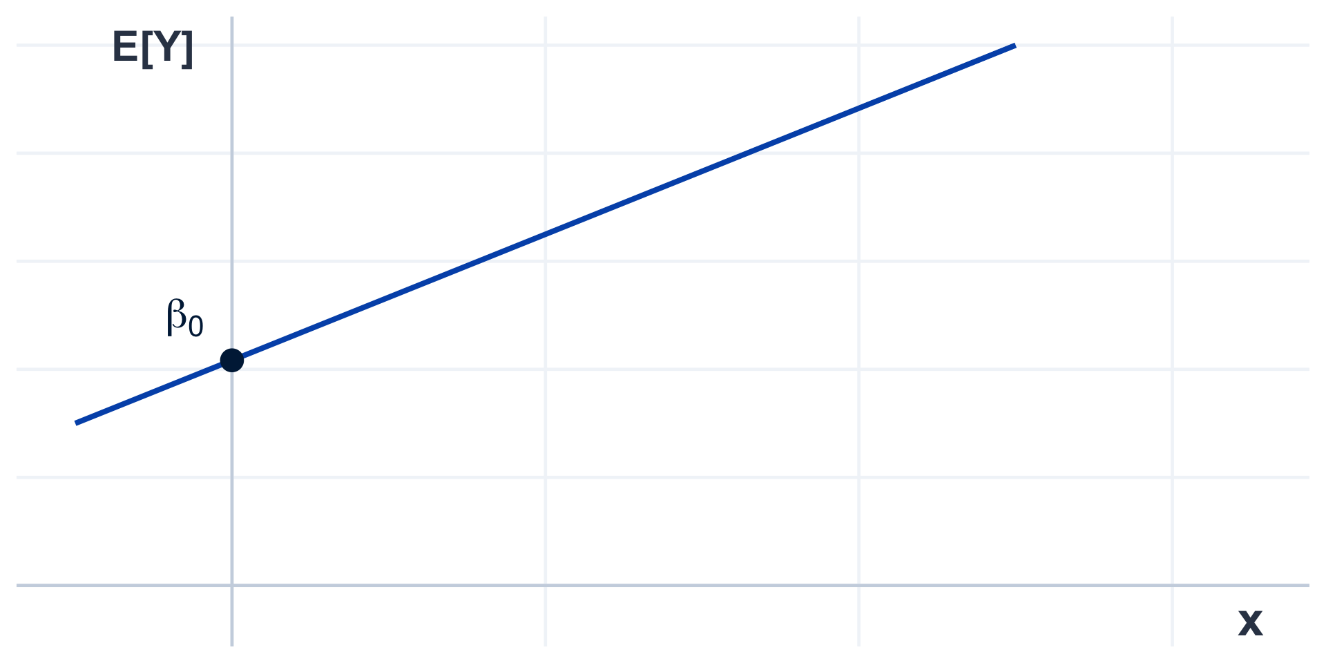
The model: components

The model relating $X$ and $Y$ is given by: \[ \mathbb{E}\left[Y_i\right] = \underbrace{\beta_0}_{\text{intercept}} + \underbrace{\beta_1}_{\text{slope}} x_i \]

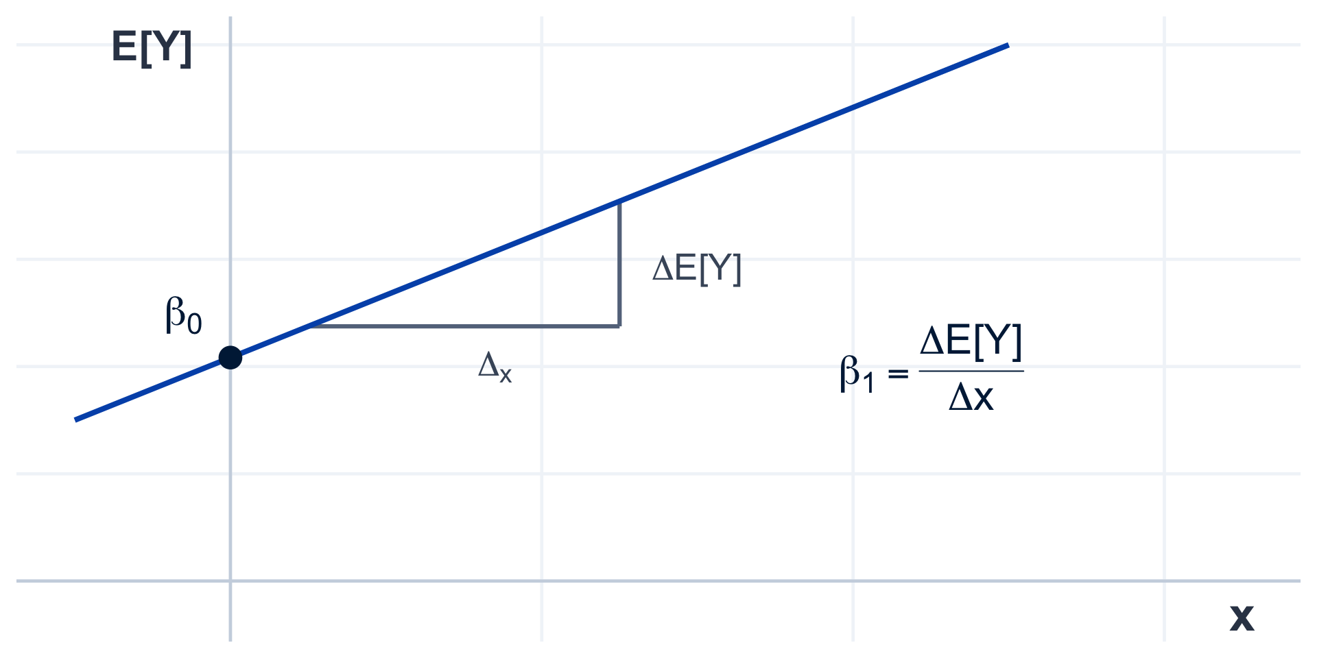
The random errors and the response

You might need to refresh this page to show the plot

Consider the following model relating the weight of a person given their height:

\[ \text{Weight} = -166+140\times\text{Height}+\varepsilon \]

For a $1.63 \text{m}$ tall person, we have:

\[ \begin{aligned} \text{Weight} &= -166 + 140 \times 1.63 + \varepsilon \\ &= 62.2 + \varepsilon \end{aligned} \]

We expect this person to weigh around $62.2\text{ kg}$;
- However, body weight is influenced by many other factors;
- Therefore, we cannot predict their exact weight with certainty.

We have a probability distribution of possible weights for a $1.63\text{ m}$ tall person:

viewof height = Inputs.range([1.4, 2.1], 
                             {
                                value: 1.63,
                                step: .01, 
                                label: "Height: ",
                                width: 400
                             });
  
viewof sigma = Inputs.range([.1, 8], 
                             {
                                value: 3,
                                step: .1, 
                                label: "σ: ",
                                width: 400
                             });

{
const mean = -166+140*height;
const stdDev = sigma;
const elementId = 'normal-density';
const title = `Weight Distribution for a person who is ${height} metres tall.`;
const xlab = 'Weight (kg)';
const ylab = 'Density';
const titleFontSize = '22px';
const labelFontSize = '18px';
const tickFontSize = '16px';
const margin = { top: 40, right: 20, bottom: 50, left: 70 };

d3_createNormalDensityPlot({
    elementId,
    mean,
    stdDev,
    title,
    xlab,
    ylab,
    titleFontSize,
    labelFontSize,
    tickFontSize,
    margin
});
}

Modelling the average

For a $1.63\text{ m}$ tall person, we have:

\[ \text{Weight} = 62.2 + \varepsilon \]

We would expect this person to weigh around $62.2\text{ kg}$;
- Some people will weigh more, and some will weigh less.
On average, $1.63\text{ m}$ tall people weigh $62.2\text{ kg}$;
- The line $−166+140\times\text{Height}$ gives the mean $\text{Weight}$ of people of a given $\text{Height}$;

The model: line vs. point

Note the difference:

\[ \overbrace{\color{red}{\underbrace{\beta_0+\beta_1 x_i}_{\text{Regression Line}:\\\quad \mathbb{E}[Y_i]}} + \epsilon_i}^{\text{Point: } Y_i} \]

The model: line vs. point

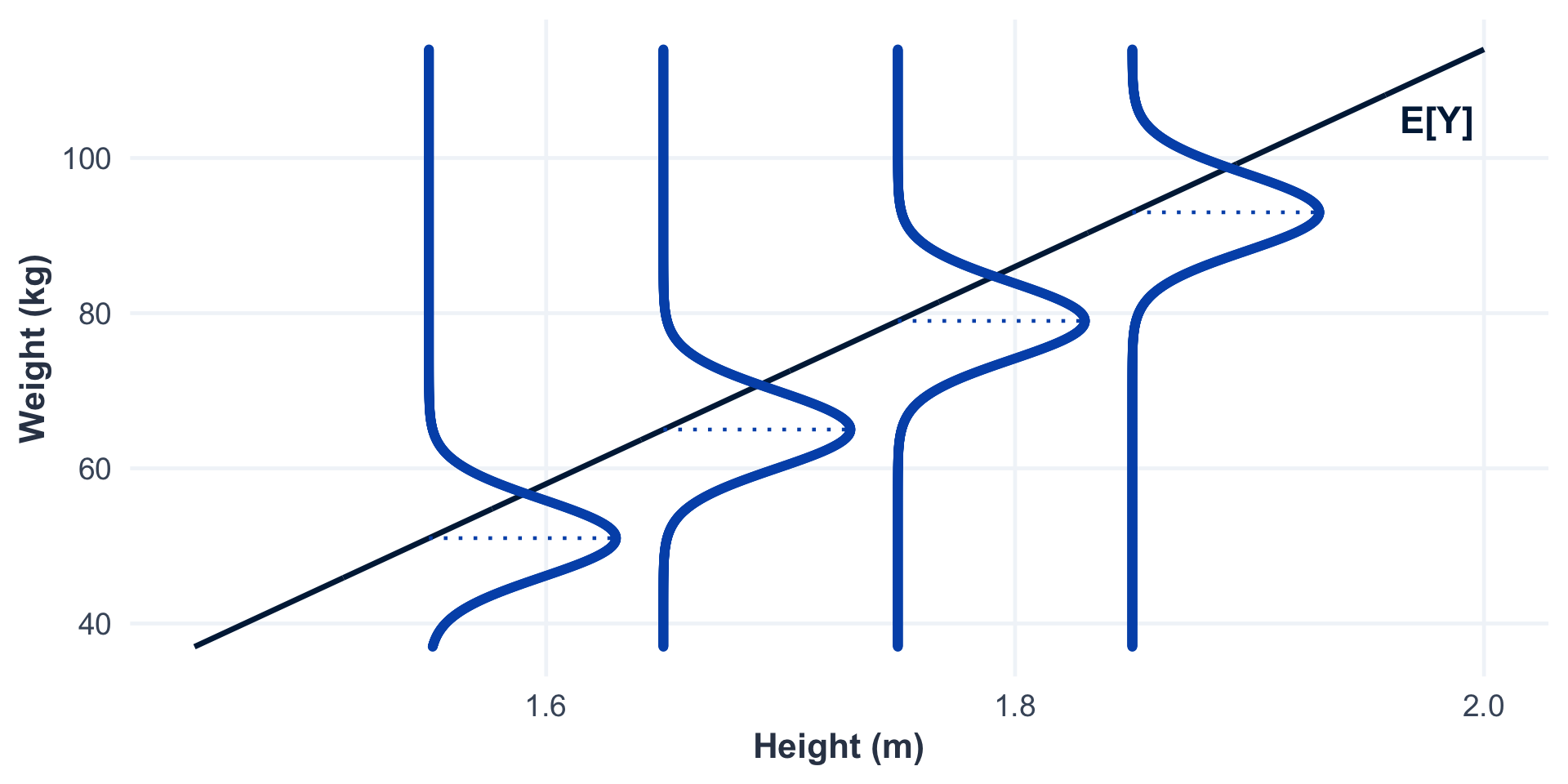
Model Fitting

Fitting is estimation

$\mathbb{E}[Y] = \beta_0 + \beta_1 x$ is the population mean of $Y$ at the fixed value $x$.
If we had repeated measurements for each value of $X=x$, we could estimate the mean for each value of $X$ separately, just by taking the average of the $Y$ values for each value of $X$.

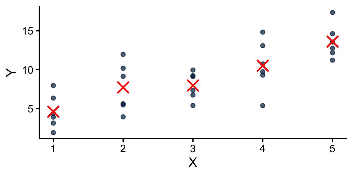
Figure 1: Repeated $Y$ observations for a few fixed values of $X$; red X’s mark the sample mean of $Y$ at each $X$.

Fitting is estimation

In general, we don’t have repeated measurements for each value of $X$:

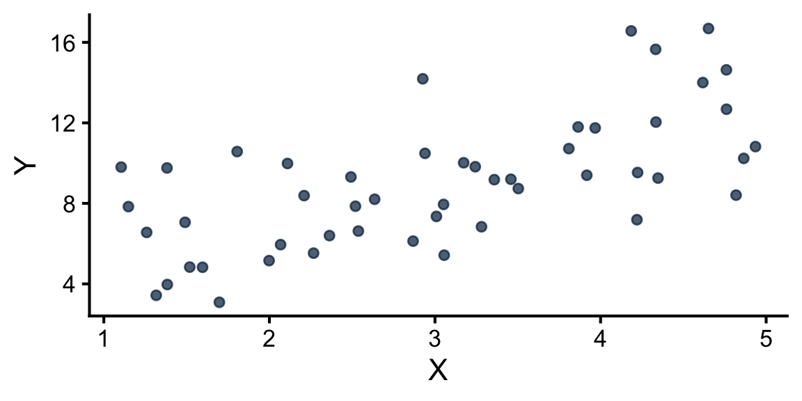
Figure 2: A single $Y$ observation for each value of $X$; we cannot estimate the mean of $Y$ at each $X$ separately.

Fitting is estimation

In fact, there are regions with no observed $X$ whatsoever:

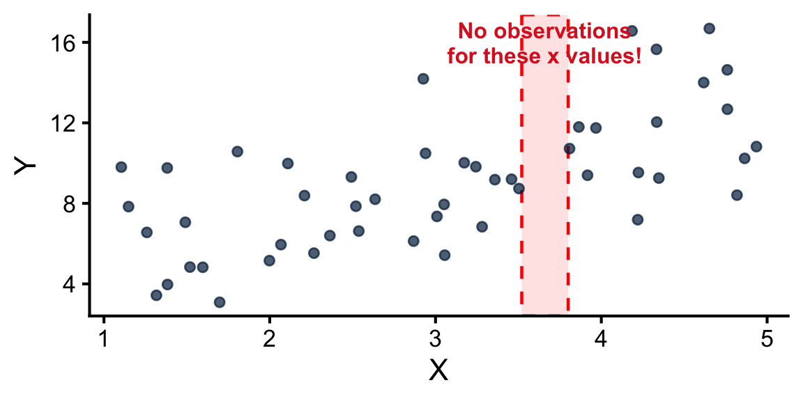
Figure 3: Regions with no data. Estimating $\mathbb{E}[Y]$ separately at each point is completely impossible without a structural model.

Linear structure

So, estimating the mean for each value of $X$ separately is not feasible.

But, what if we assume a linear structure between the mean of the population and the value of $X$?
The estimation of the means $\mathbb{E}[Y]$ for all values of $X$ reduces to estimating $\beta_0$ and $\beta_1$.
We denote the estimators by $\widehat{\beta}_0$ and $\widehat{\beta}_1$.

Fitting the model using R

To fit a linear model in R, we use the lm function.

So, the estimated values of the parameters are $\widehat{\beta}_0 = -5872.09$ and $\widehat{\beta}_1 = 50.15$.

Interpretation of $\beta_0$ and $\beta_1$

Slope ($\beta_1$): A one-unit increase in $X$ is associated with an expected change of $\beta_1$ units in $Y$.
- This is an association, not a causal effect!
Intercept ($\beta_0$): The expected value of $Y$ when $X = 0$.
- Often an extrapolation with no meaningful physical interpretation (e.g., zero flipper length or zero height).

Important: Association is not causality.

In general, we cannot conclude that changes in $X$ cause a change in $Y$. The conclusion of causality requires more than a good model.

Interpretation of $\beta_0$ and $\beta_1$

This means that an increase of $1\text{ mm}$ in flipper length is associated with an expected increase of $50.15\text{ g}$ in body mass.
Not ok to say: “An increase of $1\text{ mm}$ in flipper length increases body mass by $50.15\text{ g}$.”

Predicting with the model

To predict the value of $Y$ for a given $x$, we use the estimated regression line: \[ \widehat{Y} = \widehat{\beta}_0 + \widehat{\beta}_1 x \]
$\widehat{Y}$ is called the predicted value.

For example, we expect that a penguin with a flipper length of 200mm has a body mass of: \[\widehat{Y} = 50.15 \times 200 - 5872.09 = 4157.91g\]

Predicting in R: `predict()`

The predict() function receives as input the fitted model and new observations for which we want to predict the response value.

The new observations must be provided as a data.frame whose column names match the model formula.
- Passing a raw number like predict(model, 200) will not work.

Common Pitfall: newdata

If you omit the newdata argument or misname it, R will silently ignore the new data and use the original training data instead.
- For example, predict(model, data = new_penguin) returns all 344 fitted values ($\widehat{Y}_i$) with no error or warning!
- This is a very common and often confusing mistake;

We can also predict for multiple values at once:

The Range Problem

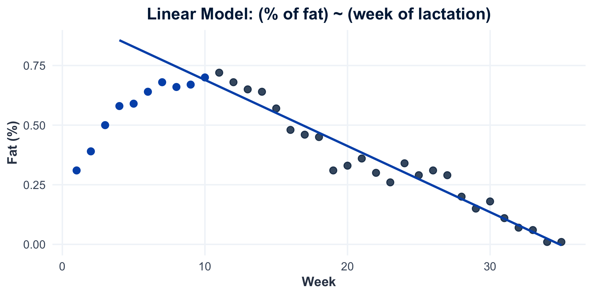
The linear model assumes that the relationship between $X$ and $\mathbb{E}[Y]$ is linear, which may or may not be true;

Sometimes, there’s a linear association only in part of the data range.
- The linear model could still be useful when restricted to that specific range;

The Range Problem

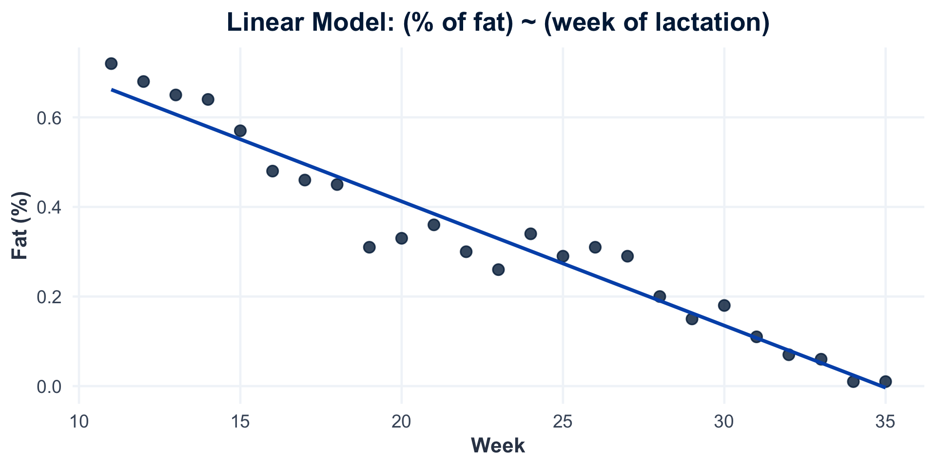
According to our model, what is the fat percentage after week 36?

The Range Problem

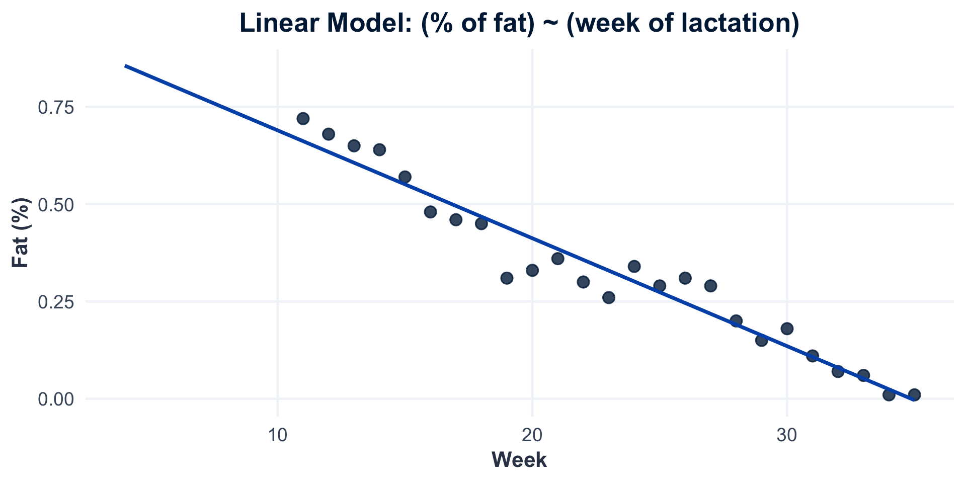
According to our model, what is the fat percentage before week 11?

The Range Problem

Let’s look at the actual data before week 11:

The Range Problem: Take-away

There’s no way for us to know whether the relationship is still linear outside the range of the data;
Be cautious when using the model outside the range of the data, as the relationship between $X$ and $Y$ may differ significantly.

Regression vs Correlation Analysis

Correlation analysis: we’re interested in the strength of linear association between two variables;
- no distinction between the two variables (no response and no covariate);
- both variables are assumed to be stochastic;

Linear Regression: we’re interested in estimating the average value of the response at each fixed value of the covariate.
- covariate is assumed to be non-stochastic;
- one of the variables is treated as a response and the other as a covariate;

Categorical Covariates

Encoding problem

Suppose that instead of flipper_length_mm we want to use the sex of penguins to explain their body_mass_g. Our model then is:

\[ \text{body_mass_g}_i = \beta_0 + \beta_1\text{sex}_i + \varepsilon_i \]

But wait! How can we have categories in an equation?

Two common encodings for categorical variables are:
1. One-hot-encoding: very common in ML applications
2. Dummy variables: very common in Statistics

One-hot-encoding (2 categories)

A categorical variable with $C$ categories will be encoded using $C$ variables.
The penguins’ sex can be male or female. Then,

\[ x_{i}^{\text{(male)}} = \begin{cases} 1 & \text{if penguin } i \text{ is male}\\ 0 & \text{otherwise} \end{cases}\qquad x_{i}^{\text{(female)}} = \begin{cases} 1 & \text{if penguin } i \text{ is female}\\ 0 & \text{otherwise} \end{cases} \]

The model becomes

\[ Y_i = \beta_0 + \beta_1 x_{i}^{\text{(male)}} + \beta_2 x_{i}^{\text{(female)}} + \varepsilon_i \]

One Hot Encoding: Problem

But note that one hot encoding is redundant:

If you tell me what $x_{i}^{\text{(male)}}$ is, I’ll know what the value of $x_{i}^{\text{(female)}}$ is.
- So, I don’t need both in my model!

Redundant variables in linear regression cause problems:
- there are infinitely many possible solutions for $\widehat{\beta}_0$, $\widehat{\beta}_1$ and $\widehat{\beta}_2$.

Dummy variables

A categorical variable with $C$ categories will be encoded using $C - 1$ variables.
- A variable with two categories needs only 1 dummy variable.
For example, the variable $\text{sex}_{i}$ could be defined as:

\[\begin{equation} \text{sex}_i = \begin{cases} 1 & \text{if penguin $i$ is male}\\ 0 & \text{if penguin $i$ is female} \end{cases} \end{equation}\]

A variable patient_status could be defined:

\[\begin{equation} \text{patient_status}_i = \begin{cases} 1 & \text{if patient $i$ is sick}\\ 0 & \text{if patient $i$ is healthy} \end{cases} \end{equation}\]

Activity: Dummy Variables and Regression Coefficients

Consider the following model: \[ Y_i=\beta_0 + \beta_1 \text{sex}_i + \varepsilon_i,\qquad \begin{equation} \text{sex}_i = \begin{cases} 1 & \text{if penguin $i$ is male}\\ 0 & \text{if penguin $i$ is female} \end{cases} \end{equation} \]

What is the Expected Value of $Y$ given that the penguin is male?
What is the Expected Value of $Y$ given that the penguin is female?
Use the above to explain the meaning of $\beta_0$ and $\beta_1$ in this model.

Solution

For a male penguin ($\text{sex}_i = 1$), we have: \[ \begin{align*} \mathbb{E}[Y_i] &= \beta_0 + \beta_1 \times \text{sex}_i\\ &= \beta_0 + \beta_1 \times 1\\ &= \beta_0 + \beta_1 \end{align*} \]
Similarly, for a female penguin ($\text{sex}_i = 0$), we have: \[ \begin{align*} \mathbb{E}[Y_i] &= \beta_0 + \beta_1 \times \text{sex}_i\\ &= \beta_0 + \beta_1 \times 0\\ &= \beta_0 \end{align*} \]
$\beta_0$ is the expected value of $Y$ when the penguin is female, and $\beta_1$ is the difference in expected values of $Y$ between male and female penguins.

Dummy Variables

The model becomes: \[Y_i = \beta_0 + \beta_1 \text{sex}_i + \varepsilon_i\]
Let $\mu_{\text{male}} = \mathbb{E}[Y_i]$ for a male penguin ($\text{sex}_i=1$), and $\mu_{\text{female}} = \mathbb{E}[Y_i]$ for a female penguin ($\text{sex}_i=0$). Then: \[ \begin{align} \mu_{\text{male}} &= \beta_0 + \beta_1\\ \mu_{\text{female}} &= \beta_0 \end{align} \]
Therefore, \[\beta_1 = \mu_{\text{male}} - \mu_{\text{female}}\] is the difference in expected values of $Y$ between male and female penguins.

Dummy Variable: Fitting the model

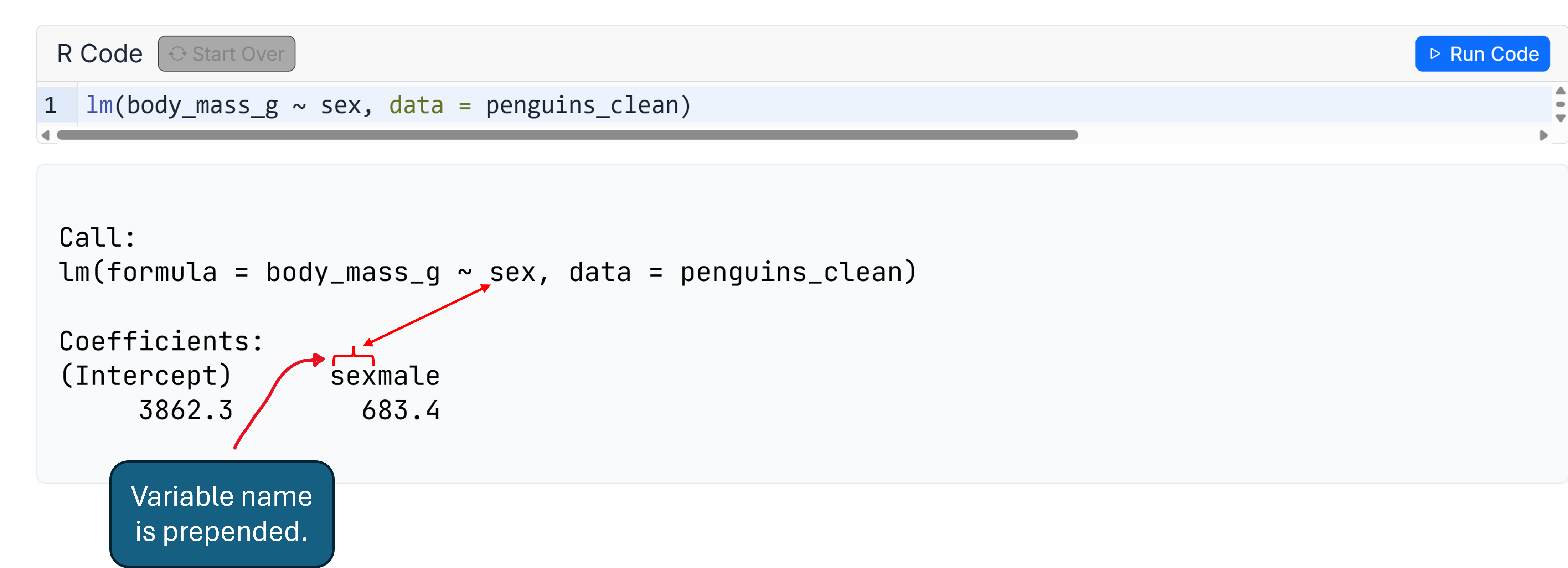
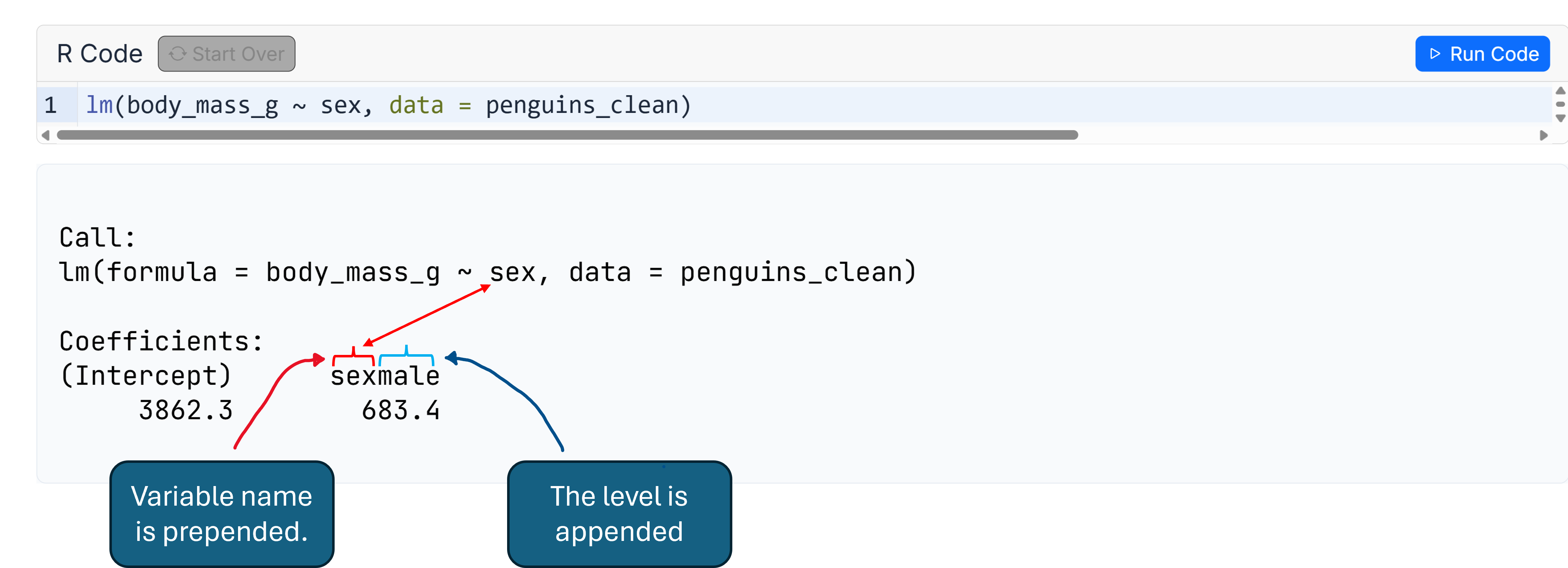
$\widehat{\beta}_0 = 3862.3$ is the estimated average body_mass_g of female penguins.

$\widehat{\beta}_1 = 683.4$ is the estimated difference in average body_mass_g between male and female penguins.
- the average weight of male penguins is $\widehat{\beta}_0+\widehat{\beta}_1 = 4545.7$

Let’s take a look at the sample statistics:

Where is the line?

Note that there is no line in this case.
Sex cannot be 0.1 or 0.5. It can only be 0 or 1.
So, what is going on?

\[\begin{equation} \text{body_mass_g}_i = \begin{cases} \beta_0 + \beta_1 + \varepsilon_i& \text{if penguin $i$ is male}\\ \beta_0 + \varepsilon_i & \text{if penguin $i$ is female} \end{cases} \end{equation}\]

We are just comparing means

Remember that in regression, we model the mean given the value of a covariate.
So, in this case, we are modelling the mean of female penguins and the mean of male penguins;
Note that:
- $\beta_0$ is the average body_mass_g of female penguins.
- $\beta_1$ is the difference in means.
- $\beta_0+\beta_1$ is the average body_mass_g of male penguins.

Population vs Sample Regression

Population Regression: \[ Y_i = \beta_0 + \beta_1 x_i + \varepsilon_i \]
Sample Regression (estimated from the sample): \[ Y_i = \widehat{\beta}_0 + \widehat{\beta}_1 x_i + e_i \]

Note that $e_i\neq\varepsilon_i$ because $\widehat{\beta}_0\neq \beta_0$ and $\widehat{\beta}_1\neq \beta_1$

The parameters $\beta_0$ and $\beta_1$

Since $\beta_0$ and $\beta_1$ are unknown population parameters, we estimate them based on a sample;
$\widehat{\beta}_0$ and $\widehat{\beta}_1$ are the estimators of $\beta_0$ and $\beta_1$.
But how do we find the “best” estimates for a given sample?

Take-home points

Simple Linear Regression Model: \[Y_i = \beta_0 + \beta_1 x_i + \varepsilon_i\] decomposes the response into a systematic mean line \[\mathbb{E}[Y_i] = \beta_0 + \beta_1 x_i\] and a random error $\varepsilon_i \sim (0, \sigma^2)$ with zero mean, constant variance, and uncorrelated errors ($\text{Cov}(\varepsilon_i, \varepsilon_j) = 0$).
Parameter Interpretation:
- Intercept $\beta_0$: expected value of $Y$ when $x = 0$
  - often an extrapolation without practical meaning.
- Slope $\beta_1$: expected change in $Y$ associated with a 1-unit increase in $x$.
- Association is not causality: regression quantifies statistical relationships, not causal mechanisms.
The Range Problem (Extrapolation):
- Predictions are only reliable within the range of observed predictor data.
- Extrapolating beyond the data range assumes linearity without evidence.
Categorical Covariates:
- A binary predictor is represented using a single dummy variable.
- $\beta_0$ represents the mean of the reference group.
- $\beta_1$ is the difference in group means.
Population vs. Sample:
- True parameters $\beta_0, \beta_1$ and true errors $\varepsilon_i$ are unobservable. We estimate them using sample statistics $\widehat{\beta}_0, \widehat{\beta}_1$
- Residuals $e_i = y_i - \widehat{y}_i \neq \varepsilon_i$.

Looking Ahead

How do we choose the optimal line through our sample data?
In this module, we just relied on R to fit the model and estimate the parameters.
In Module 02, we formalize the Least Squares Criterion and derive the formulas for the estimators $\widehat{\beta}_0$ and $\widehat{\beta}_1$.

Simple Linear Regression

Learning Objectives

Linear Models

Specification

The model

The model: components

The random errors

Exercises: Basic Properties of our model

iClicker: Question 2.1

iClicker: Question 2.1 Answer

iClicker: Question 2.2

iClicker: Question 2.2 Answer

iClicker: Question 2.3

iClicker: Question 2.3 Answer

iClicker: Question 2.4

iClicker: Question 2.4 Answer

The model: components

The model: components

The model: components

The random errors and the response

Modelling the average

The model: line vs. point

The model: line vs. point

Model Fitting

Fitting is estimation

Fitting is estimation

Fitting is estimation

Linear structure

Fitting the model using R

Interpretation of \(\beta_0\) and \(\beta_1\)

Interpretation of \(\beta_0\) and \(\beta_1\)

Predicting with the model

Predicting in R: predict()

The Range Problem

The Range Problem

The Range Problem

The Range Problem

The Range Problem: Take-away

Regression vs Correlation Analysis

Categorical Covariates

Encoding problem

One-hot-encoding (2 categories)

One Hot Encoding: Problem

Dummy variables

Activity: Dummy Variables and Regression Coefficients

Solution

Dummy Variables

Dummy Variable: Fitting the model

Dummy Variable: Fitting the model

Dummy Variable: Fitting the model

Dummy Variable: Fitting the model

Where is the line?

We are just comparing means

Population vs Sample Regression

The parameters \(\beta_0\) and \(\beta_1\)

Take-home points

Looking Ahead

Predicting in R: `predict()`