(Under construction) Sampling Distributions

Learn how samples connect to populations, understand sampling variability through simulation, discover the Central Limit Theorem, and master bootstrapping with interactive R examples.

Learning objectives

• Define and distinguish population, sample, parameter, and statistic, and give examples of each.

• Distinguish between the population distribution, the sample distribution, and the sampling distribution.

• Explain why sampling variability exists and why it is a fundamental challenge for statistical inference.

• Describe the key properties of a sampling distribution: center (bias), spread (standard error), and shape.

• State the Central Limit Theorem (CLT) and explain when it applies in practice.

• Use simulation to empirically build and explore a sampling distribution.

• Use the bootstrap method to approximate the sampling distribution from a single sample.

• Use the infer package in R to compute bootstrap distributions and confidence intervals.

Introduction

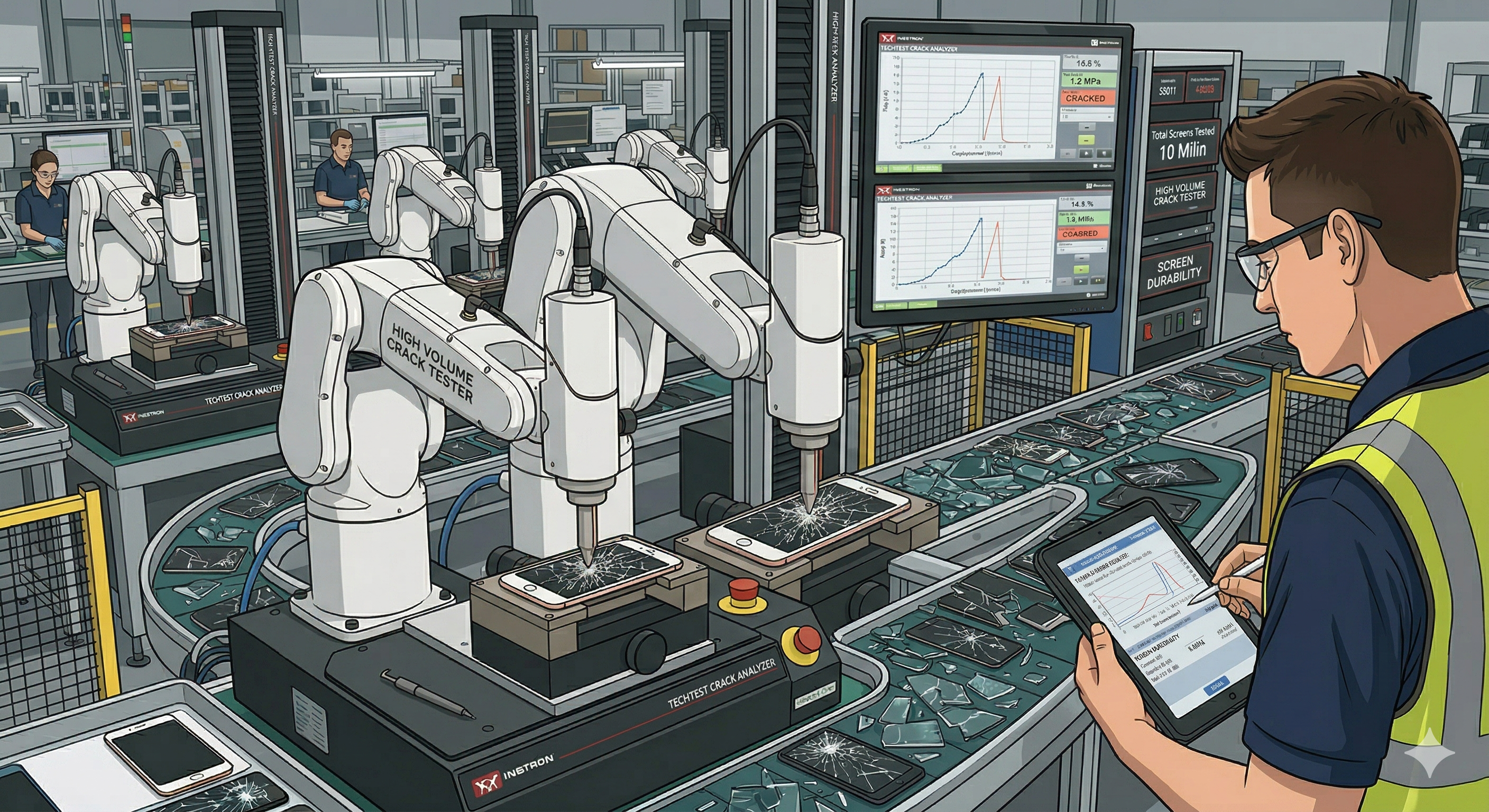
Imagine you are a quality-control manager at Apple’s iPhone manufacturing plant. Apple sources its displays from external suppliers, and every incoming shipment must meet strict durability standards before it goes into production. A new shipment of \(50{,}000\) screens has just arrived. To verify quality, you need to determine the average pressure at which a screen cracks — if the average falls below the required threshold, the shipment goes back to the supplier.

Screen durability testing: Applying pressure until the screen cracks.

Exercise 1 How would you approach this problem?

The most straightforward answer to Exercise 1 is to test every screen. If you did, you would know exactly the cracking pressure of every unit and could answer any durability question with perfect certainty. There is just one problem: testing a screen destroys it. Test all \(50{,}000\) and you have no screens left to assemble iPhones — a flawless quality report, and no product to ship.

So, how can we learn (at least approximately) about the average pressure at which the screens crack without testing all the screens?

A reasonable solution is to test a portion of the screens (i.e., a sample) and use what we learn from that sample to make an informed decision about the whole shipment. This is the essence of statistical inference: learning about a large population from a smaller, manageable sample.

But going down this path raises important questions:

1. How should you select the screens to be tested?
2. How many screens is enough?
3. How confident can you be that what you observed in, say, \(300\) screens reflects the behaviour of all \(50{,}000\)?
4. If a colleague independently tested a different \(300\) screens, would they reach the same conclusion?

These questions are of fundamental importance in any statistical study, and they are not just technical details — because statistical inference is not about making educated guesses; it is about quantifying uncertainty in a rigorous, principled way so that decisions can be made with a known level of confidence.

In this tutorial, we build the conceptual foundations of statistical inference from the ground up. By the end, you will understand not just which statistics to compute, but why they work and how much to trust them.

1 Population and Parameters

In statistical inference, we generalize the information from a sample to the entire population. In everyday conversation, words like “population,” “sample,” and “inference” are used quite loosely. To be able to statistically generalize our results, we must be absolutely clear about the boundaries of our study: Who are we studying? What are we measuring?

In statistics, giving these concepts exact boundaries is what allows us to make safe, reliable calculations. Let’s establish these core building blocks, always keeping our shipment of screens in mind.

1.1 Who are we studying? The target population.

The first thing to nail down is the group we care about. In the screens problem, Apple’s decision is about the shipment that just arrived — all \(50{,}000\) screens sitting in the warehouse. We call this group the target population:

Definition 1 (Target Population) The complete group of all individuals or items that we are interested in studying.

The boundary of the target population matters more than it might seem. It is specifically this shipment, not every screen the supplier has ever made, and not next month’s delivery. A conclusion about this population does not automatically transfer to any other. Defining the target population carefully is the first — and often most overlooked — step of any study.

Example 1 Imagine a social media company wants to study user satisfaction. They define their target population simply as “our users.” But what exactly is a “user”?

• Is it anyone who has ever registered an account?
• Is it only “monthly active users” (anyone who logged in at least once in the last 30 days)?
• Or is it only “power users” who spend at least 1 hour on the app daily?

How they resolve this ambiguity completely changes the scope of the study:

• If they include anyone who ever registered, the population will be filled with millions of abandoned accounts, diluting the data.
• If they limit it to daily power users, they will study a highly engaged “survivor” group, completely missing the opinions of people who rarely log in because they are unhappy.

□

As you can see in the example above, a vague population boundary doesn’t just make your calculations messy — it can lead to dangerously misleading business decisions.

1.2 What do we measure? The variable of interest.

Once we know who we are studying, we specify what we want to learn about each element. In the screens problem, we want to know the pressure at which each screen cracks. We call this the variable of interest:

Definition 2 (Variable of Interest) The characteristic or measurement we wish to study.

In our problem, the variable is crack pressure (in psi). Screen #1 has its own crack pressure, screen #2 has a different one, and so on for all \(50{,}000\) screens. In summary, each element in the population has their own value for the variable of interest.

Note that crack pressure is a numerical variable — i.e., it is a number, and taking averages or comparing pressures makes sense. Not every variable works this way. If we were instead asking each screen “did it pass or fail quality control?”, the variable would be categorical — it places each screen into one of two groups rather than assigning it a number.

ImportantCommon Mistake: Count vs. Variable

Students often think: “If we count that 480 screens passed, ‘480’ is a number, so shouldn’t this be a numerical variable?”

Remember to always look at the individual level. The variable is what you record for one single screen. If you walk up to Screen #42, its value is simply a category: "pass" or "fail". The fact that we later count or average these categories doesn’t change the nature of the variable itself. If the individual raw data consists of labels/words, the variable is categorical.

The type of variable matters because it determines which summaries and statistical methods are appropriate. We will see both types throughout the course.

Exercise 2 For each of the following scenarios, identify the type of the variable of interest at the individual level.

(a) An agricultural scientist measures the weight (in grams) of individual apples harvested from an orchard.

viewof answer_sd_var_a = Inputs.radio(
  ["Numerical — weight is measured on a continuous numerical scale, and averages or differences are meaningful.",
   "Categorical — weight just places apples into groups like small, medium, or large."],
  {label: "Variable type: "}
)

(b) A biology department records the natural hair color (e.g., black, brown, blonde, red) of students enrolled in an introductory course.

viewof answer_sd_var_b = Inputs.radio(
  ["Numerical — we can count how many students have each hair color.",
   "Categorical — hair color is a descriptive label, placing each student into a category."],
  {label: "Variable type: "}
)

(c) A university registrar records each student’s phone number.

viewof answer_sd_var_c = Inputs.radio(
  ["Numerical — phone numbers consist entirely of digits.",
   "Categorical — phone numbers act as labels/identifiers; performing mathematical operations (like averaging) on them makes no sense."],
  {label: "Variable type: "}
)

1.3 What if we could measure everything? Population distribution and parameters.

If we could somehow afford to measure the crack pressure of every screen in the shipment (without destroying them), we would have a complete list of \(50{,}000\) numbers, one per screen. This complete picture is called the population distribution:

Definition 3 (Population Distribution) The collection of values of the variable of interest across the entire population.

(Disclaimer: this is not a formal definition of “distribution”, but it will serve us well throughout the course.)

With the population distribution in hand, we could answer any question about the shipment:

• What fraction of screens crack below Apple’s \(750\) psi threshold? If it is more than \(1\%\), Apple returns the shipment.
• What is the average crack pressure across all \(50{,}000\) screens?
• What pressure can \(99.9\%\) of screens withstand?
  • This could be useful for warranty purposes: if we know that \(99.9\%\) of screens survive at least \(X\) psi, we can offer a warranty covering any screen that cracks under \(X\) psi.

Unfortunately, the population distribution is precisely what we cannot observe directly. In this case, measuring crack pressure requires applying pressure until the screen breaks — it is a destructive test. Measure all \(50{,}000\) and you have zero screens left to put in iPhones.

This is not just a quirk of the screens problem. In virtually every real study, the population distribution is unobservable — because measuring the entire population is too expensive, too slow, ethically impossible, or, as here, physically destructive. The whole point of statistical inference is to learn something reliable about the population distribution from a small, observable piece of it.

For learning purposes, let’s play pretend. Suppose we have access to the entire shipment of \(50{,}000\) screens’ crack pressure data. In practice, we would never have access to this; but having the ground truth here let us study how well our statistical methods work.

A histogram let us see the overall shape — where the values concentrate, how much spread there is, and whether the distribution is symmetric or skewed.

We can see that the distribution is right-skewed (i.e., a longer tail on the right), meaning some screens are exceptionally strong — and that most screens survive well above the \(750\) psi threshold. But a small fraction (just left of the red line) do not.

Making sense of a list with \(50{,}000\) values is not easy, so having a list of \(50{,}000\) numbers is not useful in itself. What matters are specific numerical summaries that let us answer our questions — like the fraction of screens that crack below Apple’s \(750\) psi threshold, or the average crack pressure across the shipment. These numerical summaries of the population distribution are called parameters.

Definition 4 (Parameter) A numerical summary of the population distribution.

Parameters describe the population as a whole; they are fixed (constants) but usually unknown. Common parameters include the proportion \(p\), the mean \(\mu\), the median \(Q_{0.5}\), and the standard deviation \(\sigma\). The right choice depends on the question. For example, for the screens shipment:

• “What fraction of screens fail Apple’s threshold?” → proportion \(p\)
  • the fraction of all \(50{,}000\) screens with crack pressure below \(750\) psi.
     
• “What is the typical crack pressure?” → mean \(\mu\) or median \(Q_{0.5}\)
  • these are central tendency measures; the median might be more informative here because the distribution is slightly right-skewed — a few extremely strong screens would inflate the mean without reflecting the typical screen. But more importantly, it gives us a very useful interpretation: “Half of the screens crack below \(Q_{0.5}\) psi, and half above.” The mean would be harder to interpret in this context.
     
• “How consistent is the manufacturing process?” → standard deviation \(\sigma\)
  • a small \(\sigma\) means screens are uniform; a large \(\sigma\) means quality varies widely. It is related to the width of the distribution — a wider distribution has a larger \(\sigma\).
     
• “What pressure can \(99.9\%\) of screens withstand?” → quantile \(Q_{0.001}\)
  • the \(0.1\)th percentile, useful for setting warranty thresholds.

Parameters are much easier to communicate than a raw list of \(50{,}000\) numbers. Compare:

“I’m returning this shipment because \(3.2\%\) of screens crack under \(750\) psi, and our standard requires no more than \(1\%\).”

versus

“I’m returning this shipment — here are the \(50{,}000\) crack-pressure values I collected. I don’t like them.”

The first message is immediately clear, yet it doesn’t mention the raw values at all. The second is useless, even though it contains all the data. At some point, we need to summarize the population distribution to make informed decisions.

CautionVariable vs. parameter: a common confusion

Students very frequently confuse variables for parameters and vice-versa. The variable is what you measure on each individual screen — screen #3,471 has a crack pressure of \(803.2\) psi; screen #12,847 has \(941.7\) psi. Every screen has its own value. The parameter is a single number that summarizes the entire population — \(p = 0.032\) is the fraction of all \(50{,}000\) screens that fail. One lives at the level of the individual; the other lives at the level of the population.

1.3.1 Exercises

Exercise 3 A streaming platform wants to understand whether its users are engaging enough with the service. The business team asks: does the average daily watch time across all active subscribers exceed \(45\) minutes?

(a) What is the variable of interest, and is it numerical or categorical?

viewof answer_sd_1_1_a = Inputs.radio(
  ["The average daily watch time across all subscribers (numerical)",
   "Each subscriber's daily watch time, in minutes (numerical)",
   "Whether each subscriber watched more than 45 minutes that day (categorical)",
   "The total number of minutes streamed platform-wide (numerical)"],
  {label: "Variable of interest: "}
)

(b) What is the parameter of interest, and what symbol do we use for it?

viewof answer_sd_1_1_b = Inputs.radio(
  ["The watch time of the subscriber who watches the most (no standard symbol)",
   "The average daily watch time across all active subscribers (μ)",
   "The proportion of subscribers who exceed 45 minutes (p)",
   "The standard deviation of watch times (σ)"],
  {label: "Parameter: "}
)

Exercise 4 What proportion of screens in the shipment crack at or below \(750\) psi? Is this above or below Apple’s \(1\%\) maximum?

TipHint

In R, a comparison like x <= threshold returns TRUE for each element that satisfies the condition and FALSE otherwise. How would you turn a vector of TRUE/FALSE values into a proportion?

TipSolution

screens_pop |>
  summarise(proportion = mean(crack_pressure <= 750))

Exercise 5 What pressure can \(99.9\%\) of the screens in the shipment withstand? (That is, find the pressure such that only \(0.1\%\) of screens crack at or below it.)

TipHint

If \(99.9\%\) of screens survive at or above a pressure, what fraction crack below it? Which percentile does that correspond to? R has a function that computes percentiles directly — check ?quantile if you’re unsure of the syntax.

TipSolution

screens_pop |>
  summarise(pressure = quantile(crack_pressure, 0.001))

Exercise 6 Samsung’s sales representative pushes back:

“Look the average crack pressure for this shipment is around \(1{,}000\) psi — well above your \(750\) psi threshold. There’s no way this shipment fails your standard.”

Is the representative’s argument convincing?

viewof answer_sd_1_4 = Inputs.radio(
  ["Yes — a mean of 1,000 psi is far above 750 psi, so the failure rate must be negligible.",
   "No — even with a high average, the population can have many screens below 750 psi.",
   "It depends — we need to know the standard deviation before deciding.",
   "Yes — the mean is the only parameter that matters for threshold decisions."],
  {label: "Your answer: "}
)

2 Sample

In the previous section, we established what we want to learn: the target population, the variable of interest, and the parameters that concisely describe the population distribution. But, since we cannot measure the variable of interest for every individual in the population, we collect data on a subset of the population: a sample. In this section, we introduce some new concepts: what a sample is, how to draw one to avoid systematic bias, how to summarize the data it contains, and how those summaries connect back to the parameters we actually care about. Let’s start with the definition of a sample.

Definition 5 (Sample) A subset of the population.

What we hope for is that this subset will represent the population well, but this is not always the case.

1. Imagine you are making a soup and want to know if it has enough salt. You don’t drink the whole pot; you taste a single spoonful (a sample) and extrapolate your finding to the entire pot (the population). If you stirred the pot well before tasting, the spoonful will be a great representation of the whole pot of soup.

2. Now imagine you are cooking a basket of french fries. You take a single piece to see if you have put enough salt. But, purely by random chance, you grab a fry on top of the basket that got too much salt on top. You conclude incorrectly that the whole basket is too salty. Here, you drew a random sample that doesn’t represent the population well (but it is still a sample)!

Soup tasting: Homogeneous mixing represents the population well.

French fries: Outliers in solid mixtures can lead to unrepresentative samples.

The french fries example makes this crystal clear: a sample is not necessarily representative — the word “sample” simply means a subset of the population, and carries no guarantee of quality. But the situation is even trickier than that: since we do not know the population distribution, we can never be certain whether our sample is a “good” one (i.e., represents the population well) or a “bad” one (unrepresentative).

Because we cannot assess the quality of individual samples, how we draw our samples becomes crucial. We need to develop good sampling methods that are reliable and allow us to measure our uncertainty in a principled way.

2.1 How do we sample? Simple Random Sampling

In statistics, there are many possible sampling strategies, each with its own advantages and disadvantages. Some of the most common include:

• Simple random sampling: every member of the population has an equal chance of being selected.
• Stratified sampling: the population is divided into subgroups (strata), and a random sample is drawn from each.
• Cluster sampling: the population is divided into clusters, and clusters are randomly selected.

All of these methods share one key ingredient that makes them effective: randomness.

Randomness is the magical element of statistics — and it may feel counterintuitive at first. How can randomness be a good thing? Isn’t it better to be precise and deliberate? Well, to start with, randomness prevents the hand-picking that introduces bias in sample selection by ensuring that no individual or subgroup is systematically favoured or excluded. In addition, it gives us the mathematical tools to quantify how uncertain our estimates are — something no non-random method can do in a principled way.

In this course, we focus exclusively on simple random sampling (SRS). Don’t let the name fool you. SRS is a widely used method in practice, and it is surprisingly good given how “simple” it is. There are two types of SRS: with replacement and without replacement.

To draw a simple random sample of size \(n\) without replacement from a population, you:

1. List all elements of the population.
2. Select one element at random (all elements have the same probability of being selected).
3. Record the selected element’s value and remove it from the population.
4. Repeat steps 2 and 3 exactly \(n\) times.

To draw a simple random sample of size \(n\) with replacement, you follow the same procedure but do not remove the selected element from the population in Step 3. Let’s explore the difference between the two methods in the next exercise.

Exercise 7 (Explore: With vs. Without Replacement) Suppose we have a population consisting of a bag of \(N = 8\) colored, numbered balls. We want to select a random sample of size \(n = 6\). Using the interactive simulator below, draw a sample under both schemes and observe how the two methods behave.

Instructions:

1. Click the “Draw next ball” button to draw balls one by one.

2. Watch the “Population (bag)” on the left (With Replacement) and the right (Without Replacement).

3. Draw all 6 balls, then answer the questions below.

mutable rwr_draw_state = ({
  sampleWith:    [],
  sampleWithout: [],
  remaining:     [0,1,2,3,4,5,6,7],
  nDrawn:        0,
  lastWith:      null,
  lastWithout:   null
})

{
  const MAX_DRAWS = 6;
  const state  = rwr_draw_state;
  const COLORS = [
    "#e05252","#e5834e","#e0be45","#6fc94f",
    "#4eb8e5","#4e78e5","#8b4ee5","#c44eb8"
  ];

  function ballHTML(idx, { grayed = false, highlighted = false, size = 40 } = {}) {
    const opacity = grayed ? 0.18 : 1.0;
    const border  = highlighted ? "3px solid #1a1a1a" : "2px solid rgba(0,0,0,0.12)";
    const shadow  = highlighted
      ? "0 0 0 3px rgba(255,255,255,0.8), 0 0 12px rgba(0,0,0,0.5)"
      : "0 2px 4px rgba(0,0,0,0.18)";
    return (
      `<span style="display:inline-flex;align-items:center;justify-content:center;` +
      `width:${size}px;height:${size}px;border-radius:50%;background:${COLORS[idx]};` +
      `color:white;font-weight:700;font-size:${size <= 32 ? 12 : 14}px;border:${border};` +
      `box-shadow:${shadow};opacity:${opacity};margin:3px;` +
      `text-shadow:0 1px 2px rgba(0,0,0,0.25);flex-shrink:0;">${idx + 1}</span>`
    );
  }

  const bagWithHTML = [0,1,2,3,4,5,6,7]
    .map(i => ballHTML(i, { highlighted: i === state.lastWith }))
    .join("");

  const bagWithoutHTML = [0,1,2,3,4,5,6,7]
    .map(i => ballHTML(i, {
      grayed:      !state.remaining.includes(i),
      highlighted: i === state.lastWithout
    }))
    .join("");

  const noDrawsMsg =
    `<span style="color:#bbb;font-size:0.82em;line-height:36px;">No balls drawn yet</span>`;

  const sampleWithHTML = state.sampleWith.length === 0 ? noDrawsMsg
    : state.sampleWith.map((i, pos) =>
        ballHTML(i, { size: 36, highlighted: pos === state.sampleWith.length - 1 })
      ).join("");

  const sampleWithoutHTML = state.sampleWithout.length === 0 ? noDrawsMsg
    : state.sampleWithout.map((i, pos) =>
        ballHTML(i, { size: 36, highlighted: pos === state.sampleWithout.length - 1 })
      ).join("");

  const hasDuplicate  = state.sampleWith.length > new Set(state.sampleWith).size;
  const duplicateBall = hasDuplicate
    ? [...state.sampleWith].find((v, i, arr) => arr.indexOf(v) !== i)
    : null;
  const canDraw = state.nDrawn < MAX_DRAWS && state.remaining.length > 0;

  const activeBtn = (color) =>
    `padding:8px 18px;background:${color};color:white;border:none;border-radius:6px;` +
    `cursor:pointer;font-size:13.5px;font-weight:600;`;
  const disabledBtn =
    "padding:8px 18px;background:#adb5bd;color:white;border:none;border-radius:6px;" +
    "cursor:not-allowed;font-size:13.5px;font-weight:600;";
  const bagBox =
    "display:flex;flex-wrap:wrap;justify-content:center;align-items:center;" +
    "padding:8px;border:1px dashed #d0d0d0;border-radius:8px;min-height:54px;" +
    "background:var(--bs-light-bg-subtle,#f8f9fa);";
  const dupMsg = hasDuplicate
    ? `<div style="text-align:center;color:#c0392b;font-size:0.88em;font-weight:600;margin-top:10px;">` +
      `⚠ Ball ${duplicateBall + 1} was drawn more than once — this can only happen with replacement!</div>`
    : "";
  const limitMsg = (!canDraw && state.nDrawn >= MAX_DRAWS)
    ? `<div style="text-align:center;color:#888;font-size:0.83em;margin-top:6px;">` +
      `Maximum draws reached. Click Reset to start over.</div>`
    : "";

  const widget = html`<div style="margin:16px 0;">
    <div style="display:flex;margin-bottom:12px;align-items:stretch;">

      <div style="flex:1;padding:16px;border:2px solid #3498db;border-radius:12px;margin:0 8px;background:var(--bs-body-bg,#fff);min-width:0;">
        <h4 style="text-align:center;margin:0 0 12px;color:#3498db;font-size:0.97em;">
          Sampling <em>With</em> Replacement
        </h4>
        <div style="font-size:0.78em;color:#888;margin-bottom:4px;text-align:center;">Population (bag)</div>
        <div style="${bagBox}">${bagWithHTML}</div>
        <div style="text-align:center;font-size:1.5em;color:#bbb;line-height:1.8;">↓</div>
        <div style="font-size:0.78em;color:#888;margin-bottom:4px;text-align:center;">
          Sample drawn so far (n&nbsp;=&nbsp;${state.nDrawn})
        </div>
        <div style="${bagBox};min-height:48px;">${sampleWithHTML}</div>
        <div style="font-size:0.75em;color:#3498db;margin-top:8px;text-align:center;">
          Each ball is <strong>returned</strong> to the bag before the next draw.
        </div>
      </div>

      <div style="flex:1;padding:16px;border:2px solid #e67e22;border-radius:12px;margin:0 8px;background:var(--bs-body-bg,#fff);min-width:0;">
        <h4 style="text-align:center;margin:0 0 12px;color:#e67e22;font-size:0.97em;">
          Sampling <em>Without</em> Replacement
        </h4>
        <div style="font-size:0.78em;color:#888;margin-bottom:4px;text-align:center;">Population (bag)</div>
        <div style="${bagBox}">${bagWithoutHTML}</div>
        <div style="text-align:center;font-size:1.5em;color:#bbb;line-height:1.8;">↓</div>
        <div style="font-size:0.78em;color:#888;margin-bottom:4px;text-align:center;">
          Sample drawn so far (n&nbsp;=&nbsp;${state.nDrawn})
        </div>
        <div style="${bagBox};min-height:48px;">${sampleWithoutHTML}</div>
        <div style="font-size:0.75em;color:#e67e22;margin-top:8px;text-align:center;">
          Each ball is <strong>removed</strong> from the bag after being drawn.
        </div>
      </div>

    </div>
    <div style="display:flex;justify-content:center;align-items:center;gap:14px;flex-wrap:wrap;">
      <button id="rwr-draw-btn" style="${canDraw ? activeBtn('#0284c7') : disabledBtn}">
        Draw next ball
      </button>
      <span style="font-size:13px;color:#666;">${state.nDrawn} / ${MAX_DRAWS} draws</span>
      <button id="rwr-reset-btn" style="${activeBtn('#6c757d')}">↺ Reset</button>
    </div>
    ${dupMsg}
    ${limitMsg}
  </div>`;

  widget.querySelector("#rwr-draw-btn").addEventListener("click", () => {
    if (!canDraw) return;
    const s          = rwr_draw_state;
    const idxWith    = Math.floor(Math.random() * 8);
    const rem        = s.remaining;
    const pickPos    = Math.floor(Math.random() * rem.length);
    const idxWithout = rem[pickPos];
    mutable rwr_draw_state = {
      sampleWith:    [...s.sampleWith, idxWith],
      sampleWithout: [...s.sampleWithout, idxWithout],
      remaining:     rem.filter((_, i) => i !== pickPos),
      nDrawn:        s.nDrawn + 1,
      lastWith:      idxWith,
      lastWithout:   idxWithout
    };
  });

  widget.querySelector("#rwr-reset-btn").addEventListener("click", () => {
    mutable rwr_draw_state = {
      sampleWith:    [],
      sampleWithout: [],
      remaining:     [0,1,2,3,4,5,6,7],
      nDrawn:        0,
      lastWith:      null,
      lastWithout:   null
    };
  });

  return widget;
}

(a) Run the simulation a few times. What is a key consequence of sampling with replacement that can never occur when sampling without replacement?

viewof answer_srs_sim_a = Inputs.radio(
  ["You can draw the exact same individual multiple times, leading to duplicate values in your sample.",
   "You can never draw the exact same individual twice.",
   "The population size decreases after each draw.",
   "The sample size is allowed to exceed the population size."],
  {label: "Consequence: "}
)

(b) Based on your observations, which sampling method is more efficient for gathering new information about a population?

viewof answer_srs_sim_b = Inputs.radio(
  ["Sampling with replacement, because keeping the population unchanged preserves the true probabilities.",
   "Sampling without replacement, because each drawn individual is guaranteed to be a new, unique member of the population.",
   "They are equally efficient because both are random."],
  {label: "More efficient method: "}
)

(c) Suppose we decide to draw a simple random sample of size \(n = 8\) with replacement, what will the resulting sample look like?

viewof answer_srs_sim_c = Inputs.radio(
  ["It will contain duplicates of some balls while missing others, just like sampling with replacement.",
   "It will consist of exactly the same 8 balls as the population.", 
   "Impossible to tell because the sample is random. It could be anything."],
  {label: "Without replacement (n = N): "}
)

In SRS with replacement, we can select the same element multiple times (because the element is not removed from the population). If we select the same element more than once, we don’t learn anything new about the population from those repeated selections. Hence, sampling with replacement is less efficient than sampling without replacement. Therefore, we always use sampling without replacement when sampling from the population.

So, why did we discuss sampling with replacement at all?

As it turns out, sampling with replacement has a key advantage: it doesn’t change the population after each draw — giving us an independent sample.

Independent sample is another key concept assumed by most statistical methods we will learn in this course. A sample is independent if the selection of one element does not affect the selection of any other element. As it turns out, SRS without replacement yields a sample that is not strictly independent, because once we select an element, it is removed from the population, which slightly changes the probabilities for the remaining elements.

Ok, so if the sample without replacement violates the assumption of independence, which we need, why did we discuss it at all?

Fortunately, if the population size, \(N\), is much larger than the sample size, \(n\), (e.g., \(N > 10n\)), the violation of independence is negligible, and we can treat the sample as “approximately independent” for practical purposes (although, technically speaking, there’s no such thing as “approximately independent”). Let’s see an example.

Example 2 Consider a box with \(6\) balls, \(3\) red and \(3\) blue.

We want to draw a sample of size \(n = 3\) balls without replacement. Let’s check the probability that the third ball is red:

First two balls selected	Chance the third ball is red
Blue, Blue	\(3/4 = 0.750\)
Blue, Red	\(2/4 = 0.500\)
Red, Red	\(1/4 = 0.250\)

As you can see, the probability of drawing a red ball on the third draw depends on what we drew in the first two draws. This means that the draws are not independent (i.e., the outcome of one draw affects the probabilities of the next draw).

But let’s check what happens when we have a much larger population with the same proportion of red balls. Say our box has \(10{,}000\) balls, where \(5{,}000\) are red and \(5{,}000\) are blue. We want to draw a sample of size \(n = 3\) balls without replacement. The probability that the third ball is red is:

First two balls selected	Chance the third ball is red
Blue, Blue	\(5{,}000/9{,}998 \approx 0.5001\)
Blue, Red	\(4{,}999/9{,}998 = 0.5000\)
Red, Red	\(4{,}998/9{,}998 \approx 0.4999\)

Again, the probabilities differ based on the first two draws, so the draws are not strictly independent, but the change in probabilities is very small. If we assume independence in our calculations, these tiny changes wouldn’t affect our results in any meaningful way. For this reason, in practice, if the sample size is small relative to the population size, we can treat the draws as independent even when sampling without replacement. How small is “small”? A common rule of thumb is that if the population size is at least 10 times larger than the sample size (\(N > 10n\)).

□

NoteRules of Thumb in Statistics

In this course, I will share several widely used “rules of thumb” with you. Many authors (myself included) disagree with some of these rules, as they are often generic and highly subjective. The \(N > 10n\) guideline above is one such examples.

Nonetheless, I will present them because they are common in practice and can be helpful for quick, initial checks. Just remember: these are guidelines, not mathematical laws, and you should always apply them with caution.

Let us return to our running example, and draw a random sample of \(n = 300\) screens from the shipment of \(50{,}000\). We will use the slice_sample() function from the dplyr package to draw our sample. (Note: remember, our population of screens is stored in the screens_pop data frame).

At this point, we have a sample of \(300\) screens. In practice, we would only have access to the data in screens_sample, and we would not know the true population distribution (which is stored in screens_pop).

Now that we have our sample, how do we use the sample to learn about the population distribution and its parameters?

2.2 Sample distribution and statistics

Think of your sample as all the information you have about the population. The information is not perfect (because it is just a small piece of the population), but it is all you have to work with. So, if you are interested in the population distribution, the best you can do is to look at the distribution of the variable of interest within your sample. This is what we call the sample distribution.

Definition 6 (Sample Distribution) The distribution of the variable of interest within a given sample.

The sample distribution is something we can observe and plot, but it changes every time we take a new sample because the sample is random. The population distribution, by contrast, is fixed (it never changes, since the population is fixed) but it is unobservable.

Once again, the sample distribution is not the same as the population distribution and it can look quite different from the population distribution (depending on the random sample you take). On the bright side, as the sample size increases, the sample distribution tends to look more and more like the population distribution. Let’s explore this convergence in action!

Exercise 8 (Explore: Effect of Sample Size on the Sample Distribution) Use the interactive simulator below to draw random samples of different sizes \(n\) from the screen durability population (screens_pop), and observe how the sample distribution behaves relative to the true population distribution.

Instructions:

1. Set the sample size (\(n\)) slider to a small value (like \(n = 10\)). Click “↺ New sample” multiple times. Notice how much the blue histogram (sample distribution) changes with each click, and how different it looks from the red line (population distribution).

2. Now, increase the slider to a large value (like \(n = 1000\) or \(n = 2000\)). Click “↺ New sample” a few times. Observe the shape of the blue histogram and the calculated sample statistics (\(\bar{x}\) and the \(\%\) below threshold).

3. Answer the questions below.

mutable cvg_state = ({ n: 100, seed: 1 })

{
  // Population parameters match screens_pop: rlnorm(meanlog=6.9, sdlog=0.15)
  const MEANLOG = 6.9, SDLOG = 0.15, THRESHOLD = 750;
  const BIN_WIDTH = 30, X_MIN = 550, X_MAX = 1700;
  const W = 660, H = 400;
  const margin = { top: 74, right: 24, bottom: 56, left: 60 };

  // Mulberry32 PRNG — deterministic, seeded
  function mulberry32(seed) {
    let a = seed | 0;
    return () => {
      a = (a + 0x6D2B79F5) | 0;
      let t = Math.imul(a ^ (a >>> 15), 1 | a);
      t = (t + Math.imul(t ^ (t >>> 7), 61 | t)) ^ t;
      return ((t ^ (t >>> 14)) >>> 0) / 4294967296;
    };
  }

  // Box-Muller log-normal sample; same seed → first n obs are identical as n grows
  function sampleLogNormal(n, seed) {
    const rng = mulberry32(seed);
    const out = [];
    for (let i = 0; i < n; i++) {
      const u1 = Math.max(rng(), 1e-10), u2 = rng();
      out.push(Math.exp(MEANLOG + SDLOG * Math.sqrt(-2 * Math.log(u1)) * Math.cos(2 * Math.PI * u2)));
    }
    return out;
  }

  const lnPDF = x => x > 0
    ? Math.exp(-Math.pow(Math.log(x) - MEANLOG, 2) / (2 * SDLOG * SDLOG)) / (x * SDLOG * Math.sqrt(2 * Math.PI))
    : 0;

  // Standard normal CDF (Abramowitz & Stegun approximation, |error| < 1.5e-7)
  function normalCDF(z) {
    const a = [0.254829592, -0.284496736, 1.421413741, -1.453152027, 1.061405429];
    const p = 0.3275911, sign = z < 0 ? -1 : 1;
    const xv = Math.abs(z) / Math.sqrt(2);
    const t = 1 / (1 + p * xv);
    const erf = 1 - ((((a[4]*t + a[3])*t + a[2])*t + a[1])*t + a[0]) * t * Math.exp(-xv * xv);
    return 0.5 * (1 + sign * erf);
  }

  const { n, seed } = cvg_state;
  const sample = sampleLogNormal(n, seed);

  // Histogram: proportion per bin (fraction of sample in each 30-psi interval)
  const edges = d3.range(X_MIN, X_MAX + BIN_WIDTH, BIN_WIDTH);
  const bins = d3.bin().domain([X_MIN, X_MAX]).thresholds(edges)(sample);
  const histData = bins.map(b => ({ x0: b.x0, x1: b.x1, y: b.length / n }));

  // PDF curve scaled to the same proportion-per-bin scale: P(X in [x, x+30]) ≈ f(x)·30
  const pdfData = d3.range(X_MIN, X_MAX, 3).map(xx => ({ x: xx, y: lnPDF(xx) * BIN_WIDTH }));

  // Live statistics
  const sampleMean = Math.round(d3.mean(sample));
  const fracBelow  = (sample.filter(v => v < THRESHOLD).length / n * 100).toFixed(1);
  const popMean    = Math.round(Math.exp(MEANLOG + SDLOG * SDLOG / 2));
  const popFrac    = (normalCDF((Math.log(THRESHOLD) - MEANLOG) / SDLOG) * 100).toFixed(1);

  // Scales
  const x = d3.scaleLinear().domain([X_MIN, X_MAX]).range([margin.left, W - margin.right]);
  const yMax = Math.max(d3.max(histData, d => d.y), d3.max(pdfData, d => d.y)) * 1.2;
  const y = d3.scaleLinear().domain([0, yMax]).range([H - margin.bottom, margin.top]);

  // Controls
  const sliderEl = html`<input type="range" min="10" max="2000" step="10" value="${n}"
    style="width:210px;accent-color:#0284c7;cursor:pointer;vertical-align:middle;">`;
  const nLabel = html`<span style="font-weight:700;color:#0284c7;min-width:44px;display:inline-block;text-align:right;">${n}</span>`;
  const drawBtn = html`<button style="padding:5px 15px;background:#0284c7;color:#fff;border:none;
    border-radius:6px;font-size:13px;font-weight:600;cursor:pointer;
    box-shadow:0 2px 8px rgba(2,132,199,0.22);">↺ New sample</button>`;

  sliderEl.addEventListener("input", () => { nLabel.textContent = +sliderEl.value; });
  sliderEl.addEventListener("change", () => { mutable cvg_state = ({ n: +sliderEl.value, seed }); });
  drawBtn.addEventListener("click", () => { mutable cvg_state = ({ n, seed: seed + 1 }); });

  const controls = html`<div style="display:flex;align-items:center;gap:14px;flex-wrap:wrap;margin-bottom:10px;">
    <label style="font-size:14px;font-weight:600;color:var(--bs-body-color);white-space:nowrap;">
      Sample size (n): ${nLabel}
    </label>
    ${sliderEl}
    ${drawBtn}
  </div>`;

  // SVG
  const svg = d3.create("svg").attr("width", W).attr("height", H)
    .style("font-family", "sans-serif").style("overflow", "visible");

  svg.append("text").attr("x", W/2).attr("y", margin.top - 46)
    .attr("text-anchor","middle").attr("font-size","15px").attr("font-weight","700")
    .attr("fill","var(--bs-body-color,#111)")
    .text(`Sample distribution (n = ${n}) vs. Population distribution`);

  svg.append("text").attr("x", W/2).attr("y", margin.top - 23)
    .attr("text-anchor","middle").attr("font-size","11.5px").attr("fill","#888")
    .text(`Sample mean x̄ = ${sampleMean} psi   |   Population mean μ ≈ ${popMean} psi`);

  // Histogram bars
  svg.append("g").selectAll("rect").data(histData).join("rect")
    .attr("x", d => x(d.x0) + 1)
    .attr("width", d => Math.max(0, x(d.x1) - x(d.x0) - 2))
    .attr("y", d => y(d.y))
    .attr("height", d => Math.max(0, y(0) - y(d.y)))
    .attr("fill","steelblue").attr("opacity",0.55);

  // Population PDF curve
  svg.append("path").datum(pdfData)
    .attr("fill","none").attr("stroke","tomato").attr("stroke-width",2.5)
    .attr("d", d3.line().x(d => x(d.x)).y(d => y(d.y)).curve(d3.curveBasis));

  // Sample mean line (x̄)
  svg.append("line")
    .attr("x1",x(sampleMean)).attr("x2",x(sampleMean))
    .attr("y1",margin.top).attr("y2",H-margin.bottom)
    .attr("stroke","steelblue").attr("stroke-width",2).attr("stroke-dasharray","4 4");
  svg.append("text").attr("x",x(sampleMean)+5).attr("y",margin.top+15)
    .attr("text-anchor","start").attr("font-size","11px").attr("fill","steelblue")
    .text(`x̄ = ${sampleMean}`);

  // Legend
  const lx = W - margin.right - 185, ly = margin.top + 12;
  svg.append("rect").attr("x",lx).attr("y",ly).attr("width",14).attr("height",14)
    .attr("fill","steelblue").attr("opacity",0.55);
  svg.append("text").attr("x",lx+18).attr("y",ly+11.5).attr("font-size","12px")
    .attr("fill","var(--bs-body-color,#333)").text("Sample distribution");
  svg.append("line").attr("x1",lx).attr("x2",lx+14).attr("y1",ly+30).attr("y2",ly+30)
    .attr("stroke","tomato").attr("stroke-width",2.5);
  svg.append("text").attr("x",lx+18).attr("y",ly+34).attr("font-size","12px")
    .attr("fill","var(--bs-body-color,#333)").text("Population distribution");

  // Axes
  svg.append("g").attr("transform",`translate(0,${H-margin.bottom})`).call(d3.axisBottom(x).ticks(8));
  svg.append("text").attr("x",W/2).attr("y",H-6).attr("text-anchor","middle").attr("font-size","13px")
    .text("Crack Pressure (psi)");

  svg.append("g").attr("transform",`translate(${margin.left},0)`)
    .call(d3.axisLeft(y).ticks(5).tickFormat(d3.format(".3f")));
  svg.append("text").attr("transform","rotate(-90)").attr("x",-(H/2)).attr("y",14)
    .attr("text-anchor","middle").attr("font-size","13px")
    .text("Proportion per 30-psi bin");

  const container = html`<div style="margin:8px 0 12px;"></div>`;
  container.append(controls);
  container.append(svg.node());
  return container;
}

(a) As you increase the sample size \(n\) using the slider, what happens to the shape of the sample distribution (blue histogram) relative to the population distribution (red curve)?

viewof answer_conv_a = Inputs.radio(
  ["The sample distribution fluctuates widely and shows no clear shape.",
   "The sample distribution looks more and more like the population distribution, and the sample statistics get closer to the population parameters.",
   "The sample distribution becomes much narrower than the population distribution.",
   "The sample distribution becomes completely flat."],
  {label: "Your observation: "}
)

(b) Click ↺ New sample several times first at \(n = 10\) and then at \(n = 2000\). Watch the steelblue dashed line (\(\bar{x}\)). How does the sample mean (\(\bar{x}\)) behave at these two sizes?

viewof answer_conv_b = Inputs.radio(
  ["The sample mean line (x̄) jumps around wildly between clicks at both sizes.",
   "The sample mean line (x̄) jumps around wildly when n = 10, but is very stable (sits near the center of the distribution) when n = 2000.",
   "The sample mean line (x̄) is stable when n = 10, but jumps around wildly when n = 2000.",
   "The sample mean line (x̄) never changes at either size."],
  {label: "Sample mean line behavior: "}
)

(c) As the sample size \(n\) increases from \(10\) to \(2000\), what happens to the overall spread (width) of the blue histogram?

viewof answer_conv_c = Inputs.radio(
  ["It becomes narrower and narrower, concentrating all data points near the center.",
   "It becomes wider and wider, because more random values are being included.",
   "Its width remains stable, reflecting the true variation of the population.",
   "There's substantial random variation of width even for large samples."],
  {label: "Histogram spread behavior: "}
)

□

Just as we compute summaries of the population distribution (parameters) to concisely describe it, we can also compute summaries of the sample distribution. Summaries of the sample distribution are called statistics, and they are used to estimate population parameters.

Definition 7 (Statistics, estimators, and estimates) A statistic is a numerical summary computed from sample data. When used to estimate a population parameter, a statistic is called an estimator. The specific value the estimator takes in a particular sample is called an estimate.

Remember, the population parameter is a fixed number that we want to learn about, but we cannot observe it directly. A statistic depends on the sample, which is random, so statistics are also random. Usually, we perform the same computation on our sample that we would on the population to calculate the parameter. For example, if we want to estimate the population mean, \(\mu\), we compute the sample mean \(\bar{X}\), which is the average of the variable of interest in our sample. If we want to estimate the population variance, \(\sigma^2\), we compute the sample variance \(S^2\).

For the screens shipment, let’s compute the sample mean \(\bar{X}\): the average crack pressure of the \(300\) sampled screens. We would use this value as our estimate of the unknown population mean \(\mu\).

In this case, the estimator is the sample mean \(\bar{X}\), and the estimate is the value we computed: sample_mean_cp.

2.3 Population vs. Sample: The Big Picture

Before moving to the exercises, let us consolidate everything introduced in this section. Each concept we use to describe the population has a direct counterpart in the sample.

The Group

Population

The entire collection of individuals or items that we are interested in studying.

Fixed Unobservable

➔ sampled
to obtain

Sample

The subset of the population actually selected, observed, and measured.

Random Observable

The Data Distribution

Population Distribution

The pattern and spread of values across the entire population.

Fixed Unknown

➔ approximated
by

Sample Distribution

The pattern and spread of values observed within the collected sample.

Random Observable

The Summary Measures

Parameter

A single numerical value summarizing the population distribution (e.g., population mean μ or proportion p).

Fixed Unknown

➔ estimated
by

Statistic / Estimator

A single numerical value calculated directly from the sample data (e.g., sample mean x̄ or proportion p̂).

Random Observable

Exercise 9 (Match the Population and Sample Concepts) Let’s put this mapping into practice. Suppose a transit agency wants to estimate the true proportion of all registered voters in Vancouver who support a new light rail proposal. They randomly select and contact \(1{,}000\) registered voters, and find that \(58\%\) of these surveyed voters support the proposal.

Match the corresponding population and sample concepts by dragging the cards from the Top Deck and dropping them into their correct roles in the Population or Sample columns below.

Top Deck (Drag cards from here)

Support/oppose status across registered voters in Vancouver

The 1,000 surveyed voters

The proportion of registered voters in Vancouver who support the proposal.

Support/oppose status across the 1,000 respondents of the survey.

All registered voters in Vancouver

58% of the respondents support the proposal.

Population

Spacer

Sample

0 of 3 counterparts matched

Exercise 10 (Sorting Properties) Now let’s verify if you can classify various quantities based on whether they describe the population (fixed but unknown) or the sample (random but observable).

Play the categorization game below to test your understanding.

0 of 6 cards sorted

2.4 Exercises

Exercise 11 A nutritionist is studying the daily fruit intake (in servings) of university students. She recruits \(n = 80\) students from the university cafeteria during lunch.

(a) Compute the sample mean fruit intake. This is the estimate of the population mean \(\mu\).

TipHint

Use the mean() function and select the fruit_servings column from the nutrition_sample dataset (i.e. nutrition_sample$fruit_servings).

sample_mean_fruit <- mean(nutrition_sample$fruit_servings) cat("Sample mean:", sample_mean_fruit)

sample_mean_fruit <- mean(nutrition_sample$fruit_servings)
cat("Sample mean:", sample_mean_fruit)

(b) Compute the sample median and sample standard deviation.

TipHint

Use summarise() to compute the summary statistics. Within summarise(), compute the median() and the standard deviation sd() of the fruit_servings column.

nutrition_sample |> summarise( median = median(fruit_servings), std_dev = sd(fruit_servings) )

nutrition_sample |>
  summarise(
    median  = median(fruit_servings),
    std_dev = sd(fruit_servings)
  )

(c) In this study, which of the following is a parameter?

viewof answer_sd_2_1_c = Inputs.radio(
  ["The sample mean fruit intake of the 80 students",
   "The mean fruit intake of all university students",
   "The fruit intake of student #42",
   "The standard deviation of the fruit intake of the 80 students"],
  {label: "Parameter: "}
)

Exercise 12 Below, four students each draw a random sample from the same population and compute the sample mean. Their results are: \(\bar{x}_1 = 47.3\), \(\bar{x}_2 = 51.8\), \(\bar{x}_3 = 44.9\), \(\bar{x}_4 = 49.6\).

(a) The four students all computed different estimates. Is this expected?

viewof answer_sd_2_2_a = Inputs.radio(
  ["Yes — different random samples almost always give different estimates",
   "No — all samples from the same population should give the same estimate",
   "It depends on the sample size",
   "It depends on the parameter being estimated"],
  {label: "Answer: "}
)

(b) Do any of these estimates equal the true population parameter?

We do not know — and in practice we never know whether our estimate happens to equal the true parameter exactly. This is the fundamental challenge of statistical inference. The sample estimates are (hopefully!) close to the truth, but essentially never exactly equal to it. Our job is to quantify how close they are likely to be.

Exercise 13 A political scientist surveys residents of Calgary to estimate the proportion of Calgarians who prefer cycling to driving for commuting. She recruits participants by standing outside shopping malls on weekday afternoons.

(a) What is the target population?

viewof answer_sd_2_3_a = Inputs.radio(
  ["All residents of Calgary",
   "People who shop at malls in Calgary",
   "People who commute by bicycle",
   "The participants in the survey"],
  {label: "Target population: "}
)

(b) Is there a potential problem with this study design?

Yes. The sampled population (mall visitors on weekday afternoons) is unlikely to represent all Calgary residents. People who visit malls on weekday afternoons may be retired, unemployed, or work shift jobs — groups with potentially different commuting habits than, say, 9-to-5 office workers who may never visit a mall on a weekday afternoon. The results of this survey may not generalize to all Calgarians.

Exercise 14 For each concept in the left column, use the dropdown to select its sample counterpart.

viewof match_sd_2_4_a = Inputs.select(
  ["— select —", "Sample", "Sample distribution", "Statistic / Estimate (x̄, p̂, s, ...)"],
  {label: html`<em>Population</em> &rarr;`}
)

viewof match_sd_2_4_b = Inputs.select(
  ["— select —", "Sample", "Sample distribution", "Statistic / Estimate (x̄, p̂, s, ...)"],
  {label: html`<em>Population distribution</em> &rarr;`}
)

viewof match_sd_2_4_c = Inputs.select(
  ["— select —", "Sample", "Sample distribution", "Statistic / Estimate (x̄, p̂, s, ...)"],
  {label: html`<em>Parameter (&mu;, p, &sigma;, &hellip;)</em> &rarr;`}
)

Exercise 15 (a) The population mean \(\mu\) is best described as:

viewof answer_sd_2_5_a = Inputs.radio(
  ["Fixed and unknown — we cannot directly observe it",
   "Fixed and known — it is a definite number we can look up",
   "Random (varies by sample) and unknown — it changes every time we sample",
   "Random (varies by sample) and known — we can compute it from our data"],
  {label: "The population mean μ is: "}
)

(b) The sample mean \(\bar{X}\) is best described as:

viewof answer_sd_2_5_b = Inputs.radio(
  ["Fixed (constant) and unknown — it is a single definite number",
   "Fixed (constant) and known — we can compute it from the data",
   "Random (varies by sample) and unknown — it changes but we cannot see it",
   "Random (varies by sample) and known — we compute it, but a different sample gives a different value"],
  {label: "The sample mean x̄ is: "}
)

(c) Apple’s quality-control manager uses the sample of \(300\) screens and reports: “The sample mean crack pressure is \(\bar{x} = 1{,}012\) psi, so the average crack pressure of all \(50{,}000\) screens is exactly \(\mu = 1{,}012\) psi.” What is wrong with this statement?

viewof answer_sd_2_5_c = Inputs.radio(
  ["Nothing!",
   "The sample mean is an estimate of μ, not μ itself; a different sample of 300 screens would almost certainly give a different value.",
   "The sample mean is always higher than the population mean, so μ < 1,012 psi.",
   "The sample is too small to compute a reliable mean."],
  {label: "What is wrong: "}
)

3 Sampling Distribution

In the previous section, we learned how to take a random sample and compute a statistic (e.g., sample mean) to estimate a population parameter. We also saw that, because samples are random, everything about the sample is random, including the statistic we compute from it. We call this sampling variability. Take a look at the code below and notice how two random samples yields different sample means.

Since we are using statistics (which are random) to estimate parameters (which are fixed), one could argue that any value we get from a single sample is just a lucky (or unlucky) draw, and has no relationship to the true population parameter.

Let’s think this through together! Suppose the true proportion of screens that can withstand a crack pressure of \(750\) psi or more is \(p = 0.95\). Since we cannot test all \(50{,}000\) screens, we have to rely on our single sample. But here is the catch: we already know that a different random sample would have given a different sample proportion. So, how can we possibly trust the one estimate we happen to have?

Imagine a scenario where every possible sample yielded a proportion very close to \(p = 0.95\). In that world, we could relax knowing our single estimate is definitely close to the truth. In this scenarion, there’s still sampling variability, but since all samples give sample proportions that are very close to the true proportion, the oscillation is irrelevant.

On the other hand, if different samples produced wildly different proportions, jumping everywhere say to \(0.7\) to \(0.8\) or \(0.99\), our single estimate could be miles away from the truth, and we would have no way of knowing it. In this scenario, the sampling variability is huge, and our single estimate is not reliable at all.

In practice, we are rarely in either of these extreme worlds. We are usually somewhere in between, where some samples give bad estimates (i.e., far away from the true parameter), while other samples give good estimates (i.e., close to the true parameter). But luckily, most samples give estimates that are reasonably close to the true parameter, and the bad samples that give terrible estimates are relatively rare. But how rare? Since, we cannot evaluate how good a given estimate is, we need to be able to quantify how likely it is that we get a good estimate versus a bad one.

To properly study this variability, we need to look at the distribution of the statistic (in this case the sample proportion) across all possible samples. This is called the sampling distribution and it is the central concept of statistical inference.

Definition 8 (Sampling Distribution) The distribution of a statistic (e.g., sample mean or sample proportion) computed from all possible samples of a given size \(n\) drawn from the population.

Let’s start with a small population and a small sample size, so that we can enumerate every possible sample and compute the statistic for each one. This will allow us to see the sampling distribution exactly.

Example 3 An aquarium has \(20\) fish. You are responsible for feeding them, and to determine the right amount of food you need to know the average weight. You decide to estimate the population mean by sampling \(3\) fish at random. The weights of all 20 fish in the population are shown in Table 1 (measured in decagrams, dkg).

Table 1: The weight of the 20 fish in the aquarium. (Note 1dkg = 10g).
(Population mean μ = 43.45 dkg)

Fish	Weight (dkg)	Fish	Weight (dkg)	Fish	Weight (dkg)	Fish	Weight (dkg)
Fish #1	43	Fish #6	44	Fish #11	26	Fish #16	42
Fish #2	46	Fish #7	41	Fish #12	47	Fish #17	36
Fish #3	47	Fish #8	40	Fish #13	37	Fish #18	36
Fish #4	59	Fish #9	43	Fish #14	42	Fish #19	61
Fish #5	24	Fish #10	58	Fish #15	60	Fish #20	37

With only \(20\) fish and a sample size of \(n = 3\), there are exactly \(\binom{20}{3} = 1{,}140\) possible samples we could get. The table below lists all \(1{,}140\) possible samples as well as their sample mean. Below the table, Figure 1 shows the histogram of the sampling distribution (you can click a bar in the histogram to highlight the corresponding samples in the table that would give a sample mean in that bin).

Table 2: All 1,140 possible samples sorted by fish numbers.
(Click one or more bars in the histogram below to highlight samples.)

fish_wt = [43, 46, 47, 59, 24, 44, 41, 40, 43, 58,
           26, 47, 37, 42, 60, 42, 36, 36, 61, 37]

fish_pop_mean_ojs = 43.45

// ── Generate all C(20,3) = 1140 samples ───────────────────────────────────────
all_fish_samples = {
  const rows = [];
  for (let i = 0; i < 20; i++) {
    for (let j = i + 1; j < 20; j++) {
      for (let k = j + 1; k < 20; k++) {
        const w = [fish_wt[i], fish_wt[j], fish_wt[k]];
        const m = +(w[0] + w[1] + w[2]).toFixed(2) / 3;
        rows.push({
          "Sample"            : `(#${i+1}, #${j+1}, #${k+1})`,
          "Sample mean (dkg)" : +m.toFixed(2)
        });
      }
    }
  }
  return rows;
}

// ── Mutable state ─────────────────────────────────────────────────────────────
mutable fish_sel      = []     // Array of selected bins: [{x0, x1}, ...]
mutable fish_rows_shown = 12

// ── All-samples table (3 per row, highlight on click) ─────────────────────────
{
  // Sort all 1140 samples by fish numbers (natural generation order)
  const sorted = all_fish_samples.slice();

  const sel       = fish_sel;
  const COLS      = 3;          // samples per table row
  const STEP      = 12;         // rows to add per click
  const totalRows = Math.ceil(sorted.length / COLS);   // 380 rows
  const shownRows = Math.min(fish_rows_shown, totalRows);

  // ── Style block ──────────────────────────────────────────────────────────────
  const styleBlock = html`<style>
    .ojs-samples-table {
      font-size: 13.5px !important;
      margin-top: 8px !important;
      margin-bottom: 8px !important;
      border-collapse: collapse !important;
      border: none !important;
      font-family: var(--bs-body-font-family, "Inter", -apple-system, sans-serif) !important;
    }
    
    /* Header cells styling to match Table 1 */
    .ojs-samples-table thead th {
      background-color: #2c3e50 !important;
      color: #ffffff !important;
      font-weight: 600 !important;
      font-size: 14.5px !important;
      padding: 0.8rem 1rem !important;
      border: none !important;
      white-space: nowrap !important;
      vertical-align: middle !important;
      text-align: left !important;
    }
    
    /* Center align the Mean Weight header */
    .ojs-samples-table thead th.num-col {
      text-align: center !important;
    }
    
    /* Separator header cell styling to make a solid continuous banner */
    .ojs-samples-table thead th.table-sep {
      background-color: #2c3e50 !important;
      padding: 0 !important;
      width: 16px !important;
      max-width: 16px !important;
      min-width: 16px !important;
      border: none !important;
    }

    /* Body cell styling to match Table 1 */
    .ojs-samples-table tbody td {
      padding: 0.8rem 1rem !important;
      vertical-align: middle !important;
      text-align: left !important;
      border-bottom: 1px solid rgba(0, 0, 0, 0.05) !important;
      font-size: 14px !important;
    }

    /* Center-align numeric columns in body */
    .ojs-samples-table tbody td.num-col {
      text-align: center !important;
    }

    /* Zebra striping (even rows) to match Table 1 */
    .ojs-samples-table tbody tr:nth-child(even) td:not(.lit-cell) {
      background-color: rgba(0, 0, 0, 0.015) !important;
    }
    
    /* Hover styling to match Table 1 */
    .ojs-samples-table tbody tr:hover td:not(.lit-cell) {
      background-color: rgba(0, 0, 0, 0.035) !important;
      transition: background-color 0.2s ease;
    }

    /* Highlighted cells on click */
    .ojs-samples-table td.lit-cell {
      background-color: rgba(255, 99, 71, 0.12) !important;
      color: tomato !important;
      font-weight: bold;
    }

    /* Separator body cell styling */
    .ojs-samples-table tbody td.table-sep {
      background-color: transparent !important;
      background: transparent !important;
      border: none !important;
      padding: 0 !important;
      width: 16px !important;
      max-width: 16px !important;
      min-width: 16px !important;
    }
  </style>`;

  // ── Status message ───────────────────────────────────────────────────────────
  let statusEl;
  if (sel && sel.length > 0) {
    const count = sorted.filter(
      d => sel.some(item => d["Sample mean (dkg)"] >= item.x0 && d["Sample mean (dkg)"] < item.x1)
    ).length;
    statusEl = html`<p style="color:tomato; font-weight:bold; margin:10px 0 6px;">
      ${count} sample${count !== 1 ? "s" : ""} highlighted in the selected mean intervals.
      Click a highlighted bar again to deselect, or click Reset in the histogram to clear all.
    </p>`;
  } else {
    statusEl = html`<p style="color:#555; margin:0 0 6px;">
      
    </p>`;
  }

  // ── Table header row ─────────────────────────────────────────────────────────
  const headerCells = [];
  for (let c = 0; c < COLS; c++) {
    if (c > 0) headerCells.push(html`<th class="table-sep"></th>`);
    headerCells.push(html`<th>Sampled Fish</th>`);
    headerCells.push(html`<th class="num-col">Mean Weight<br>(dkg)</th>`);
  }
  const headerRow = html`<tr>${headerCells}</tr>`;

  // ── Data rows ────────────────────────────────────────────────────────────────
  const dataRows = [];
  for (let r = 0; r < shownRows; r++) {
    const cells = [];
    for (let c = 0; c < COLS; c++) {
      const idx = r * COLS + c;
      if (c > 0) cells.push(html`<td class="table-sep"></td>`);
      if (idx < sorted.length) {
        const row  = sorted[idx];
        const mean = row["Sample mean (dkg)"];
        const lit  = sel && sel.length > 0 && sel.some(item => mean >= item.x0 && mean < item.x1);
        const cellClass = lit ? "lit-cell" : "";
        const meanClass = lit ? "lit-cell num-col" : "num-col";
        cells.push(html`<td class="${cellClass}">${row["Sample"]}</td>`);
        cells.push(html`<td class="${meanClass}">${mean}</td>`);
      } else {
        cells.push(html`<td></td>`);
        cells.push(html`<td></td>`);
      }
    }
    dataRows.push(html`<tr>${cells}</tr>`);
  }

  // ── Buttons ──────────────────────────────────────────────────────────────────
  const remaining = totalRows - shownRows;
  const btnStyle  = "padding:4px 12px; font-size:13px; cursor:pointer; margin-right:6px;";
  const btnContainer = html`<div style="margin-top:8px;">`;

  if (shownRows < totalRows) {
    const nextBatch  = Math.min(STEP, remaining);
    const showMoreBtn = html`<button style="${btnStyle}">Show ${nextBatch} more rows (${remaining} remaining)</button>`;
    showMoreBtn.addEventListener("click", () => { mutable fish_rows_shown = shownRows + STEP; });
    btnContainer.append(showMoreBtn);

    if (shownRows + STEP < totalRows) {
      const showAllBtn = html`<button style="${btnStyle}">Show all ${totalRows} rows</button>`;
      showAllBtn.addEventListener("click", () => { mutable fish_rows_shown = totalRows; });
      btnContainer.append(showAllBtn);
    }
  }

  if (shownRows > STEP) {
    const collapseBtn = html`<button style="${btnStyle}">↑ Collapse</button>`;
    collapseBtn.addEventListener("click", () => {
      mutable fish_rows_shown = STEP;
      setTimeout(() => {
        const el = document.getElementById("tbl-fish-sampling-dist");
        if (el) {
          el.scrollIntoView({ behavior: "smooth", block: "start" });
        }
      }, 50);
    });
    btnContainer.append(collapseBtn);
  }

  // ── Assemble ─────────────────────────────────────────────────────────────────
  const wrapper = html`<div></div>`;
  wrapper.append(styleBlock);
  const table = html`<table class="table ojs-samples-table">
    <thead>${headerRow}</thead>
    <tbody>${dataRows}</tbody>
  </table>`;
  wrapper.append(table);
  if (btnContainer.children.length > 0) wrapper.append(btnContainer);
  wrapper.append(statusEl);
  return wrapper;
}

viewof show_true_mean = {
  const form = html`<form style="display: inline-flex; align-items: center; margin: 0; padding: 0;">
    <label style="display: inline-flex; align-items: center; gap: 8px; margin: 0; padding: 0; cursor: pointer; user-select: none; font-size: 14.5px; font-weight: 500; color: var(--bs-body-color); line-height: 1;">
      <input type="checkbox" style="cursor: pointer; width: 16px; height: 16px; margin: 0 !important; padding: 0 !important; accent-color: #0284c7; flex-shrink: 0;">
      <span style="display: inline-block; line-height: 1;">Show population mean <span style="color:tomato; font-weight: bold;">(μ = 43.45)</span></span>
    </label>
  </form>`;
  
  const input = form.querySelector("input");
  input.addEventListener("change", () => {
    form.value = input.checked;
    form.dispatchEvent(new CustomEvent("input"));
  });
  
  form.value = false;
  return form;
}

// ── Interactive histogram ──────────────────────────────────────────────────────
{
  const sel      = fish_sel || [];
  const showMean = show_true_mean;

  const W = 640, H = 480;
  const margin = { top: 65, right: 20, bottom: 65, left: 65 };

  // Bin all 1140 sample means with a set domain to ensure equal width bins
  const thresholds = d3.range(29, 62, 2.5);
  const binner = d3.bin()
    .value(d => d["Sample mean (dkg)"])
    .domain([26, 62])
    .thresholds(thresholds);
  const bins = binner(all_fish_samples);

  const x = d3.scaleLinear()
    .domain([bins[0].x0 - 0.3, bins[bins.length - 1].x1 + 0.3])
    .range([margin.left, W - margin.right]);

  const y = d3.scaleLinear()
    .domain([0, d3.max(bins, d => d.length) + 10])
    .range([H - margin.bottom, margin.top]);

  // Create relative outer container to position the Reset Selection button inside the plot cell
  const container = html`<div style="position: relative; width: ${W}px; margin: 0 auto;"></div>`;

  const svg = d3.create("svg")
    .attr("width", W).attr("height", H)
    .style("font-family", "sans-serif").style("font-size", "13px");

  // Create premium reset button absolute positioned at the top-right
  const resetBtn = html`<button style="
    position: absolute;
    top: ${margin.top}px;
    right: ${margin.right}px;
    z-index: 10;
    padding: 6px 14px;
    font-size: 12.5px;
    font-weight: 600;
    cursor: pointer;
    border: none;
    border-radius: 6px;
    background: #0284c7; /* Vibrant modern blue */
    color: #ffffff;
    transition: background 0.15s, transform 0.15s, box-shadow 0.15s;
    box-shadow: 0 4px 12px rgba(2, 132, 199, 0.25);
  ">↺ Reset Selection</button>`;

  resetBtn.addEventListener("mouseover", () => {
    resetBtn.style.background = "#0369a1"; // Elegant deep ocean blue
    resetBtn.style.boxShadow = "0 6px 16px rgba(2, 132, 199, 0.35)";
    resetBtn.style.transform = "translateY(-1px)";
  });
  resetBtn.addEventListener("mouseout", () => {
    resetBtn.style.background = "#0284c7";
    resetBtn.style.boxShadow = "0 4px 12px rgba(2, 132, 199, 0.25)";
    resetBtn.style.transform = "translateY(0)";
  });
  resetBtn.addEventListener("click", () => {
    mutable fish_sel = [];
  });

  if (sel.length > 0) {
    container.append(resetBtn);
  }

  // Plot Title
  svg.append("text")
    .attr("x", W / 2).attr("y", margin.top - 36)
    .attr("text-anchor", "middle")
    .attr("fill", "var(--bs-body-color, #111)")
    .attr("font-size", "17px").attr("font-weight", "600")
    .style("font-family", "system-ui, -apple-system, sans-serif")
    .text("Sampling Distribution of the Sample Mean");

  // Instruction subtitle
  svg.append("text")
    .attr("x", W / 2).attr("y", margin.top - 12)
    .attr("text-anchor", "middle")
    .attr("fill", "#666").attr("font-size", "12px")
    .text("Click one or more bars to highlight samples in the table above · click again to deselect");

  // Helper: check if a bin is selected
  const isBinSelected = d => sel.some(item => item.x0.toFixed(3) === d.x0.toFixed(3));

  // Bars
  const bars = svg.append("g").selectAll("rect").data(bins).join("rect")
    .attr("x",      d => x(d.x0) + 1)
    .attr("width",  d => Math.max(0, x(d.x1) - x(d.x0) - 1))
    .attr("y",      d => y(d.length))
    .attr("height", d => y(0) - y(d.length))
    .attr("fill",   d => isBinSelected(d) ? "tomato" : "steelblue")
    .style("cursor", "pointer");

  // Count label on selected bars
  if (sel.length > 0) {
    sel.forEach(item => {
      const selBin = bins.find(d => d.x0.toFixed(3) === item.x0.toFixed(3));
      if (selBin) {
        svg.append("text")
          .attr("x", (x(selBin.x0) + x(selBin.x1)) / 2)
          .attr("y", y(selBin.length) - 5)
          .attr("text-anchor", "middle")
          .attr("font-size", "11px").attr("fill", "tomato").attr("font-weight", "bold")
          .text(selBin.length);
      }
    });
  }

  // Hover: lighten bar and show count
  bars.on("mouseover", function(event, d) {
    const isSelected = isBinSelected(d);
    if (!isSelected) d3.select(this).attr("fill", "#4a8ab5");
    if (!isSelected) {
      svg.append("text").attr("class", "hover-count")
        .attr("x", (x(d.x0) + x(d.x1)) / 2)
        .attr("y", y(d.length) - 5)
        .attr("text-anchor", "middle")
        .attr("font-size", "11px").attr("fill", "#333")
        .text(d.length);
    }
  }).on("mouseout", function(event, d) {
    const isSelected = isBinSelected(d);
    if (!isSelected) d3.select(this).attr("fill", "steelblue");
    svg.selectAll(".hover-count").remove();
  });

  // Click: toggle selection (support multi-select)
  bars.on("click", function(event, d) {
    const index = sel.findIndex(item => item.x0.toFixed(3) === d.x0.toFixed(3));
    if (index > -1) {
      // Remove from selection
      mutable fish_sel = sel.filter((_, i) => i !== index);
    } else {
      // Add to selection
      mutable fish_sel = [...sel, { x0: d.x0, x1: d.x1 }];
    }
  });

  // Population mean line (toggled)
  if (showMean) {
    svg.append("line")
      .attr("x1", x(fish_pop_mean_ojs)).attr("x2", x(fish_pop_mean_ojs))
      .attr("y1", margin.top).attr("y2", H - margin.bottom)
      .attr("stroke", "red").attr("stroke-width", 2)
      .attr("stroke-dasharray", "6 3");
    svg.append("text")
      .attr("x", x(fish_pop_mean_ojs) + 6).attr("y", margin.top + 18)
      .attr("fill", "red").attr("font-size", "12px")
      .text(`μ = ${fish_pop_mean_ojs}`);
  }

  // X axis
  svg.append("g")
    .attr("transform", `translate(0,${H - margin.bottom})`)
    .call(d3.axisBottom(x).ticks(10));
  svg.append("text")
    .attr("x", W / 2).attr("y", H - 10)
    .attr("text-anchor", "middle").attr("font-size", "14px")
    .text("Sample Mean Weight (dkg)");

  // Y axis
  svg.append("g")
    .attr("transform", `translate(${margin.left},0)`)
    .call(d3.axisLeft(y).ticks(6));
  svg.append("text")
    .attr("transform", "rotate(-90)")
    .attr("x", -(H / 2)).attr("y", 16)
    .attr("text-anchor", "middle").attr("font-size", "14px")
    .text("Count (number of samples)");

  container.append(svg.node());
  return container;
}

Figure 1: Sampling distribution of the sample mean weight across all 1,140 possible samples of 3 fish. Click a bar to highlight the corresponding samples in the table above. Click again to deselect.

□

Exercise 16 Using the interactive histogram above, answer the following questions.

(a) What is the smallest sample mean you can find? How many samples give this minimum sample mean? Which fish are in these samples?

• Smallest sample mean: 28.67 dkg (approximately 286.7 grams).
• Number of samples: 2 samples that yield this minimum mean.
  • Sample 1: (Fish #5, Fish #11, Fish #17) (weights: 24, 26, and 36 dkg)
  • Sample 2: (Fish #5, Fish #11, Fish #18) (weights: 24, 26, and 36 dkg)

The leftmost bar in the histogram corresponds to these two samples — which are among the unluckiest possible samples, giving the worst underestimates of the true population mean (\(\mu = 43.45\) dkg).

(b) Click on bars to select all samples whose mean falls between \(40\) and \(46\) dkg. How many such samples are there?

viewof answer_fish_1a = Inputs.radio(
  ["Less than 300",
   "Between 300 and 500",
   "Between 500 and 700",
   "More than 700"],
  {label: "Number of samples: "}
)

(c) Which of the following ranges is the most likely to contain the sample mean of a randomly selected sample?

viewof answer_fish_1c = Inputs.radio(
  ["29 to 39 dkg",
   "39 to 49 dkg",
   "49 to 59 dkg"],
  {label: "Range: "}
)

(d) By looking at the sampling distribution, do you have serious concerns of over- or under-estimating the true population mean \(\mu\)?

No, the sampling distribution is roughly centered around the true population mean \(\mu = 43.45\) dkg, which means that roughly half of the possible samples yield a sample mean above the correct value and half below.

□

3.1 Exploring sampling variability via simulation

We almost never get to see the sampling distribution directly in practice (that would require collecting thousands of independent samples — prohibitively expensive). But since we have an artificial population, we can simulate it.

Let’s take \(5{,}000\) different random samples of size \(n = 300\) from screens_pop, compute the sample mean \(\bar{X}\) for each, and look at the distribution of those \(5{,}000\) estimates.

1. rep_sample_n (from the infer package) draws reps random samples of size size from the data.
2. For each sample (identified by replicate), we compute the sample mean crack pressure.

Let’s visualize the sampling distribution:

Look at that! Even though individual crack pressures follow a right-skewed distribution, the sampling distribution of \(\bar{X}\) is smooth and approximately bell-shaped (Normal). This result — striking and powerful — is the Central Limit Theorem at work, which we will explore in detail in Section 5.

ImportantThree Distributions You Must Not Confuse

This is where most students stumble. There are three distributions at play, and they are entirely different things:

1. Population distribution: The distribution of the variable of interest across all individuals in the population. It is fixed but usually unknown.

2. Sample distribution: The distribution of the variable of interest in your specific sample. It is observable, but changes every time you take a new sample.

3. Sampling distribution: The distribution of the statistic (e.g., \(\hat{p}\) or \(\bar{X}\)) across all possible samples of size \(n\). It is theoretical — you can approximate it via simulation — and it describes how much your estimate varies from sample to sample.

3.2 Properties of the sampling distribution

When statisticians study a sampling distribution, they focus on three key properties.

3.2.1 Center: Bias

The center of the sampling distribution is the long-run average of the statistic across all possible samples. If this center equals the true parameter value, the statistic is said to be unbiased.

Definition 9 (Unbiased Estimator) A statistic is an unbiased estimator of a parameter \(\theta\) if the mean of its sampling distribution equals \(\theta\).

In plain English: an estimator is unbiased if it gets the right answer on average. In any single sample, your sample mean \(\bar{X}\) will probably overshoot or undershoot the true population mean \(\mu\). But if you repeated the process millions of times, the overshoots and undershoots would perfectly cancel out, and the average of all your estimates would be exactly equal to the truth. There is no systematic tendency to be too high or too low.

Let’s check whether \(\bar{X}\) is unbiased for \(\mu\):

The mean of the \(5{,}000\) simulated \(\bar{X}\) values is essentially equal to the true \(\mu\). The sample mean is an unbiased estimator of the population mean. It does not systematically over- or underestimate the truth.

3.2.2 Spread: Standard error

The spread of the sampling distribution measures how much the statistic varies from sample to sample. The standard deviation of the sampling distribution has a special, important name.

Definition 10 (Standard Error (SE)) The standard deviation of the sampling distribution of a statistic. It measures the typical amount of variation in the statistic from sample to sample.

A small standard error means the statistic is precise — different samples give very similar estimates. A large standard error means the estimates jump around a lot from sample to sample.

The theoretical formula for the standard error of \(\bar{X}\) is: \[\text{SE}(\bar{X}) = \frac{\sigma}{\sqrt{n}}\]

where \(\sigma\) is the standard deviation of the population, and \(n\) is the sample size.

This formula reveals two critical insights: 1. Population variation (\(\sigma\)): If the population itself is highly variable (large \(\sigma\)), then our sample means will also be more variable from sample to sample (larger SE). 2. Sample size (\(n\)): Because \(n\) is in the denominator, increasing the sample size reduces the standard error. This is the key lever we control: larger samples yield smaller standard errors, giving us more precise estimates.

3.2.3 Shape

Look at the histogram of the sampling distribution again — it is approximately Normal (bell-shaped), even though the population distribution is right-skewed. This happens because of the Central Limit Theorem, which we cover in Section 5.

3.3 Effect of sample size

One of the most important practical questions in statistics is: how large does my sample need to be? Let’s investigate this directly by comparing the sampling distribution of \(\bar{X}\) for different sample sizes.

viewof n_size_sd = Inputs.range([20, 2000], {
  step: 20,
  value: 200,
  label: "Sample size (n)"
})

{
  const mu    = 1000;   // population mean (screens_pop: lognormal meanlog=6.9, sdlog=0.15)
  const sigma = 151;    // population SD
  const se    = sigma / Math.sqrt(n_size_sd);
  const xMin  = mu - 5 * se;
  const xMax  = mu + 5 * se;

  const data = d3.range(xMin, xMax, (xMax - xMin) / 500).map(x => ({
    x,
    density: Math.exp(-Math.pow((x - mu), 2) / (2 * se * se)) /
             (se * Math.sqrt(2 * Math.PI))
  }));

  return Plot.plot({
    style: { fontSize: "14px" },
    marks: [
      Plot.line(data, { x: "x", y: "density", stroke: "steelblue", strokeWidth: 2.5 }),
      Plot.ruleY([0]),
      Plot.ruleX([mu], { stroke: "red", strokeDasharray: "6 3", strokeWidth: 2 }),
      Plot.text(
        [{ x: mu + 5, y: Math.max(...data.map(d => d.density)) * 0.85,
           text: `SE = ${se.toFixed(1)} psi` }],
        { x: "x", y: "y", text: "text", fontSize: 14, fill: "steelblue" }
      )
    ],
    x: { label: "Sample Mean Crack Pressure (psi)", domain: [800, 1200] },
    y: { label: "Density" },
    grid: true,
    width: 640,
    height: 380
  });
}

Figure 2: The sampling distribution of \(\bar{X}\) for different sample sizes (population: screens_pop, \(\mu \approx 1{,}000\) psi, \(\sigma \approx 151\) psi). As \(n\) increases, the distribution narrows — estimates become more precise.

As you increase \(n\) in Figure 2, the distribution becomes narrower. But notice the rate: to halve the standard error, you need to quadruple the sample size.

Why? Because of the square root in the formula (\(\text{SE} = \sigma / \sqrt{n}\)). If you want to make the Standard Error twice as small (i.e., divide it by 2), you must multiply \(n\) by \(2^2 = 4\). This is the law of diminishing returns in sampling: while larger samples are always more precise, the reward for increasing your sample size gets progressively smaller. At some point, the financial or physical cost of testing more units (or surveying more people) outweighs the tiny gain in precision.

3.4 Exercises

Exercise 17 A regional hospital system recorded the time (in minutes) each patient spent waiting in the emergency department before being seen by a physician. Across \(20{,}000\) visits logged last year, the wait time has a population mean of \(\mu = 45\) minutes and a standard deviation of \(\sigma = 20\) minutes.

We take \(3{,}000\) random samples of size \(n = 50\) and compute the sample mean for each. The results are stored in sampling_dist_wait.

(a) Simulate the sampling distribution of \(\bar{X}\) with \(n = 50\) and \(3{,}000\) repetitions.

(b) Compute the mean and standard deviation of the sampling distribution you created. Compare them to the theoretical values: the mean of the sampling distribution (denoted as \(\mu_{\bar{X}} = \mu = 45\)) and the theoretical Standard Error (\(\text{SE}(\bar{X}) = \sigma/\sqrt{n} = 20/\sqrt{50}\)).

(c) Now simulate the sampling distribution for \(n = 200\). How does the standard error change?

viewof answer_sd_3_1_c = Inputs.radio(
  ["The SE approximately doubled",
   "The SE approximately halved",
   "The SE approximately stayed the same",
   "The SE quadrupled"],
  {label: "What happened to the SE? "}
)

Exercise 18 Two researchers, Alice and Bob, study the same population. Alice uses samples of size \(n = 100\) and Bob uses samples of size \(n = 400\).

(a) If Alice’s standard error is \(\text{SE}_A = 0.05\), what is Bob’s standard error \(\text{SE}_B\)?

viewof answer_sd_3_2_a = Inputs.radio(
  ["0.10",
   "0.025",
   "0.05",
   "0.0125"],
  {label: "SE_B = "}
)

(b) How much larger is Alice’s confidence interval expected to be compared to Bob’s?

viewof answer_sd_3_2_b = Inputs.radio(
  ["4 times larger",
   "2 times larger",
   "The same size",
   "√2 times larger"],
  {label: "Width ratio: "}
)

Exercise 19 A real estate platform recorded the sale prices (in thousands of dollars) for \(25{,}000\) homes sold in a major Canadian city last year. The data are stored in home_sales_pop.

(a) Is the population distribution symmetric, left-skewed, or right-skewed?

viewof answer_sd_3_3_a = Inputs.radio(
  ["Symmetric",
   "Left-skewed (long tail to the left)",
   "Right-skewed (long tail to the right)"],
  {label: "Shape: "}
)

(b) Simulate the sampling distribution of the sample median for samples of size \(n = 40\) with \(3{,}000\) repetitions.

TipHint

Inside summarise(), replace the blank with the R function that computes the median of a numeric vector.

(c) Does the sampling distribution of the sample median look approximately Normal? Is this surprising given the shape of the population?

Yes — despite the strongly right-skewed population, the sampling distribution of the sample median converges to an approximately bell-shaped (Normal) distribution. This is not unique to the sample mean: for large enough \(n\), the sampling distributions of many statistics (including the median) tend toward Normality. The three-distribution framework — and the behaviour of the sampling distribution — applies broadly, not just when the statistic is the sample mean.

4 The Estimator as a Random Variable

Let’s take a step back and ask a question we have been quietly glossing over: why does the sample mean \(\bar{X}\) have a distribution at all?

The answer is chance. Every time we test a new batch of \(300\) screens, we get a different mix. Which specific screens end up in the sample is random — it depends on which rows slice_sample() happened to select. Because the sample is random, the statistic computed from it is also random. Its value changes from sample to sample.

This makes \(\bar{X}\) what mathematicians call a random variable.

Definition 11 (Random Variable) A random variable is a quantity whose value is the outcome of a random process — it takes different values depending on the result of a random phenomenon.

You have encountered random variables before: the result of rolling a die (which can take values 1–6), the number of heads in 10 coin flips, or the height of a randomly selected adult from a population. In each case, you do not know the value in advance — it depends on the outcome of a random trial.

\(\bar{X}\) fits this description exactly. Before drawing the sample, you do not know which \(300\) screens will be selected, so you do not know what value \(\bar{X}\) will take. After sampling, you compute a specific number — say, \(\bar{X} = 1{,}012\) psi. That specific value is called a realization (or observation) of the random variable.

This gives us an important distinction:

• The estimator — the rule “compute the sample mean from a random sample” — is the random variable. It takes a new value every time you apply it to a new sample.
• The estimate — a specific observed value like \(\bar{X} = 1{,}012\) psi — is one realization of that random variable.

The sampling distribution is the distribution of the estimator. It tells you what values \(\bar{X}\) can take and with what probability — exactly what a distribution does for any random variable.

Now, what about the true population mean \(\mu\)? Is that a random variable? No. The true mean is fixed — it is the average crack pressure of all \(50{,}000\) screens in the shipment. It does not change when you draw a new sample. The randomness is entirely in the sampling process, not in the population.

ImportantWhat is and is not a random variable here?

Quantity	Random variable?	Reason
\(\hat{p}\), the sample proportion	✓ Yes	Its value changes with each random sample
\(\bar{X}\), the sample mean	✓ Yes	Its value changes with each random sample
\(p\), the true population proportion	✗ No	Fixed; does not depend on which sample you draw
\(\mu\), the true population mean	✗ No	Fixed; does not depend on which sample you draw
\(N\), the population size	✗ No	A fixed property of the population
\(n\), the sample size	✗ No	Fixed by design before sampling begins

Why does any of this matter? Because it determines when probability statements are meaningful. When we ask “what is the probability that our estimate \(\bar{X}\) is within \(20\) psi of the truth?”, we are asking about the random variable \(\bar{X}\) — and that question makes perfect sense, since \(\bar{X}\) takes different values depending on which screens are sampled. It would be meaningless to ask “what is the probability that \(\mu = 1{,}000\) psi?” — \(\mu\) is a fixed number, not a random variable; it either equals that value or it does not.

This is also why, when we report a point estimate, we always accompany it with a measure of its variability (like the standard error or a confidence interval). A single realization tells you where the random variable landed this time — but without knowing how spread out the sampling distribution is, you have no idea how representative that single value is.

4.1 Exercises

Exercise 20 A public health researcher takes a random sample of \(250\) adults to estimate the proportion who have been diagnosed with hypertension.

(a) Which of the following quantities is a random variable?

viewof answer_sd_rv_1_a = Inputs.radio(
  ["The true proportion of adults in the country with hypertension",
   "The sample proportion of adults with hypertension among the 250 surveyed",
   "The total number of adults in the country",
   "The sample size of 250"],
  {label: "Random variable: "}
)

(b) After completing the survey, the researcher reports: “In our sample, \(22\%\) of participants have been diagnosed with hypertension.” Is this \(22\%\) a random variable, or a realization of a random variable?

viewof answer_sd_rv_1_b = Inputs.radio(
  ["A random variable — it was computed from a random sample",
   "A realization of a random variable — it is one specific observed value",
   "Neither — it is just a summary statistic"],
  {label: "The 22%: "}
)

Exercise 21 Look back at the simulation in Section 3.1, where we took \(5{,}000\) different samples of size \(n = 300\) from screens_pop and plotted the resulting \(\bar{X}\) values. Which of the following best describes what that histogram represents?

viewof answer_sd_rv_2 = Inputs.radio(
  ["The population distribution — how crack pressures are distributed across all 50,000 screens",
   "A sample distribution — the crack pressures within one specific sample of 300 screens",
   "The sampling distribution of X̄ — the distribution of the random variable 'sample mean from 300 screens'",
   "The distribution of the fixed parameter μ"],
  {label: "That histogram represents: "}
)

5 The Central Limit Theorem

We have now seen that the sampling distribution of \(\hat{p}\) looks approximately Normal, even though individual voters just say “support” or “oppose”. This is not a coincidence. It is a consequence of one of the most remarkable and important results in all of mathematics.

Definition 12 (Central Limit Theorem (CLT)) Let \(X_1, X_2, \ldots, X_n\) be a random sample of size \(n\) from a population with mean \(\mu\) and finite standard deviation \(\sigma\). Then, for large enough \(n\), the sampling distribution of the sample mean \(\bar{X}\) is approximately Normal: \[\bar{X} \;\dot{\sim}\; N\!\left(\mu,\; \frac{\sigma}{\sqrt{n}}\right)\] In other words, the sampling distribution of \(\bar{X}\) is centered at the true population mean \(\mu\), and has a standard deviation (standard error) of \(\sigma/\sqrt{n}\).

In plain terms: no matter what shape the population distribution has — Normal, skewed, bimodal, uniform, anything — the sampling distribution of the sample mean will look like a Normal distribution, as long as \(n\) is large enough.

Why does this matter so much? Because the Normal distribution is one of the most thoroughly understood distributions in mathematics. The CLT is the bridge that allows us to use tools built for the Normal distribution (like confidence intervals and z-scores) even when the original data is far from Normal.

5.1 Seeing the CLT in action

Let’s demonstrate the CLT through simulation. We will take random samples from three populations with very different shapes and see what happens to the sampling distribution of the mean.

Run the code block below to see the sampling distributions for all three populations side by side. Try changing n_clt from small values (like \(5\)) to large values (like \(100\)) and observe what happens.

The three left panels show population distributions that look nothing like a Normal distribution. The three right panels show the corresponding sampling distribution of the sample mean — and they all converge to a bell-shaped Normal curve (the red curve). The fit is almost perfect even for \(n = 30\).

NoteWhat to Look For

When you change n_clt:

• Small \(n\) (5–10): The sampling distributions for the exponential and bimodal populations still look non-Normal (they inherit some of the parent’s skewness or shape).
• Moderate \(n\) (30–50): The Normal approximation is already quite good for the exponential case, and excellent for the uniform.
• Large \(n\) (100+): All three sampling distributions are nearly indistinguishable from perfect Normal distributions.

5.2 When does the CLT apply?

The CLT is an asymptotic result — strictly speaking, it holds exactly only as \(n \to \infty\). In practice, how large \(n\) needs to be depends on the shape of the population:

• Symmetric or mildly skewed populations: \(n \geq 20\) or \(30\) is typically sufficient.
• Moderately skewed populations: \(n \geq 50\) is a safer bet.
• Highly skewed or heavy-tailed populations: \(n \geq 100\) or more may be needed.

A rough rule of thumb that is widely used is \(n \geq 30\), but this is just a guideline, not a guarantee. When in doubt, simulate.

ImportantCLT for Proportions

The CLT also applies to the sample proportion \(\hat{p}\). When the sample size is large enough, the sampling distribution of \(\hat{p}\) is approximately Normal: \[\hat{p} \;\dot{\sim}\; N\!\!\left(p,\; \sqrt{\frac{p(1-p)}{n}}\right)\]

A widely-used condition to check whether \(n\) is “large enough” for the proportion case is: \[np \geq 10 \quad \text{and} \quad n(1-p) \geq 10\]

Both conditions must hold.

Note: In real-world scenarios where the true population proportion \(p\) is unknown, we check these conditions using our sample proportion \(\hat{p}\) instead (\(n\hat{p} \geq 10\) and \(n(1-\hat{p}) \geq 10\)).

5.3 Exercises

Exercise 22 A national survey on mental health finds that \(35\%\) of young adults report experiencing moderate or high levels of anxiety. A university wants to survey a random sample of its students to study anxiety on campus.

For each of the following sample sizes, check whether the CLT conditions (\(np \geq 10\) and \(n(1-p) \geq 10\)) are met, and compute the standard error.

(a) What is the minimum sample size \(n\) for which both CLT conditions are satisfied?

viewof answer_sd_4_1_a = Inputs.radio(
  ["10",
   "29",
   "30",
   "60"],
  {label: "Minimum n: "}
)

Exercise 23 A coffee chain claims that the average wait time at its downtown location is \(\mu = 3.5\) minutes, with a population standard deviation of \(\sigma = 1.2\) minutes. The distribution of wait times is moderately right-skewed.

A consumer advocacy group plans to sample \(n = 64\) customers and record their wait times.

(a) What is the approximate distribution of the sample mean wait time \(\bar{X}\), according to the CLT?

viewof answer_sd_4_2_a = Inputs.radio(
  ["N(3.5, 1.2)",
   "N(3.5, 1.2/√64)",
   "N(3.5, 1.2²/64)",
   "The CLT does not apply because the distribution is skewed"],
  {label: "Distribution of X̄: "}
)

(b) What is the probability that the sample mean wait time exceeds \(3.8\) minutes?

NoteHint

By the CLT, \(\bar{X} \sim N(3.5, 1.2/\sqrt{64})\). To find \(P(\bar{X} > 3.8)\), use pnorm(3.8, mean = ..., sd = ...) for the left tail, and subtract from 1.

(c) Looking at Figure 2, what would happen to \(P(\bar{X} > 3.8)\) if the sample size were doubled to \(n = 128\)?

viewof answer_sd_4_2_c = Inputs.radio(
  ["It would increase — larger samples make extreme values more likely",
   "It would decrease — larger samples make the distribution narrower, so extreme values are less likely",
   "It would not change — the probability depends only on μ, not n",
   "It would decrease — larger samples shift the mean to the right"],
  {label: "Effect of doubling n: "}
)

Exercise 24 An engineer is studying the lifespan (in years) of industrial motors. The population distribution is strongly right-skewed with mean \(\mu = 12\) years and standard deviation \(\sigma = 8\) years.

(a) Use simulation to create the sampling distribution of \(\bar{X}\) for sample sizes \(n = 10\), \(n = 30\), and \(n = 100\). Plot all three distributions and comment on how they differ.

(b) For which sample size does the sampling distribution look most like a Normal distribution?

viewof answer_sd_4_3_b = Inputs.radio(
  ["n = 10",
   "n = 30",
   "n = 100",
   "None of them — this population is too skewed for the CLT to apply"],
  {label: "Most Normal: "}
)

6 Bootstrapping: Approximating the Sampling Distribution from One Sample

Everything we have done so far — drawing thousands of samples, computing thousands of statistics, building the sampling distribution — has relied on having access to the entire population. But in real life, we rarely get to test thousands of independent batches of screens. We typically have just one sample.

So here is the big question: is there any way to approximate the sampling distribution from a single sample?

The answer is yes, through a clever technique called bootstrapping.

6.1 The idea of bootstrapping

Let’s think about what the sampling distribution captures: the variability in our statistic that arises from taking different random samples from the population. Now, since we only have one sample, we cannot take another sample from the population — but we can take another sample from our sample.

The key insight is: our sample is the best approximation we have of the population. If the sample is representative of the population, then resampling from the sample — with replacement — should give us a reasonable approximation of the variability we would see if we took new samples from the population.

Here is the procedure:

1. Start with your original sample of size \(n\).
2. Draw a new sample of size \(n\) from your original sample, with replacement. Some observations will appear multiple times, others not at all. This is a bootstrap sample.
3. Compute the statistic of interest (e.g., \(\hat{p}\) or \(\bar{X}\)) for this bootstrap sample. This is a bootstrap replicate.
4. Repeat steps 2–3 many times (typically \(5{,}000\) to \(15{,}000\) times).
5. The distribution of all bootstrap replicates is the bootstrap distribution, which approximates the shape and spread of the true sampling distribution.

NoteSampling With vs. Without Replacement

The original sample is drawn from the population without replacement (each individual appears only once). Bootstrap samples are drawn from the original sample with replacement (an individual can appear multiple times). This is intentional: it allows us to mimic the randomness of drawing new samples from the population.

Why with replacement? If we resampled \(n\) observations without replacement from a sample of size \(n\), every bootstrap sample would contain the exact same data points as the original sample! The bootstrap sample mean or proportion would always be identical, showing zero variability. Sampling with replacement is what allows the data points to mix and vary, mimicking the natural variation of drawing entirely new samples from the population.

Example 4 We tested one sample of \(n = 300\) screens from the shipment. Let’s use this single sample to approximate the sampling distribution of \(\bar{X}\) via bootstrapping.

1. We resample from screens_sample with replacement (replace = TRUE), \(10{,}000\) times.
2. For each bootstrap sample, we compute the sample mean crack pressure.

The bootstrap distribution closely follows the Normal curve predicted by the CLT — this is reassuring. Crucially, the spread of the bootstrap distribution (its standard error) approximates how much \(\bar{X}\) would vary if we drew many different samples from the population. In practice, we use the bootstrap’s spread to quantify our uncertainty, not its center.

□

6.2 The infer package workflow

The infer package (Couch et al. 2021) provides a clean, consistent workflow for bootstrapping that mirrors the workflow you will see for hypothesis testing. Let’s redo the analysis above.

1. specify(response = crack_pressure) tells infer which column we’re studying.
2. generate(reps = 10000, type = "bootstrap") creates \(10{,}000\) bootstrap samples.
3. calculate(stat = "mean") computes the sample mean for each bootstrap sample.

To visualize the bootstrap distribution:

We can also extract the standard error of the bootstrap distribution — this is our estimate of how much \(\bar{X}\) varies from sample to sample.

6.3 Bootstrap confidence intervals

One of the main applications of the bootstrap distribution is computing confidence intervals — a range of plausible values for the population parameter. We will cover confidence intervals in full detail in a later tutorial, but here is a preview.

The simplest bootstrap confidence interval uses the percentile method: we take the middle \(95\%\) of the bootstrap distribution as our confidence interval.

This interval says: based on our sample of \(300\) screens, we are \(95\%\) confident that the true population mean crack pressure is between the two reported values.

NoteWhat “95% Confident” Means

The confidence level does not mean “there is a 95% chance that the true parameter is inside this specific interval.” The true parameter \(p\) is fixed; either it is in the interval or it is not. Rather, the 95% refers to the procedure: if we repeated this entire process many times (take a sample, build a bootstrap distribution, compute the interval), about 95% of the resulting intervals would contain the true parameter. More on this in the confidence intervals tutorial.

A helpful physical analogy (rings and a peg): Think of the true population parameter as a fixed peg in the ground, and your confidence interval as a ring you throw at it. The peg never moves. The ring’s position and size change with each throw (each new random sample). A 95% confidence level means that if you throw 100 rings, about 95 of them will successfully land around the peg, while 5 will miss. It does not mean the peg is moving around inside your ring!

6.4 Bootstrapping for different statistics

One of the great advantages of bootstrapping is its flexibility: it works for virtually any statistic, not just the mean. Back to the screens problem: instead of estimating the average crack pressure \(\mu\), suppose Apple wants to estimate the proportion of screens in the shipment that fall below the \(750\) psi threshold — the parameter \(p\) that directly determines whether the shipment is accepted.

Example 5 From our single sample of \(n = 300\) screens, let’s bootstrap the proportion below the threshold.

The same four-step infer workflow — specify, generate, calculate, then extract the CI — works unchanged. The only difference is the statistic we ask for.

□

6.5 Exercises

Exercise 25 A random sample of \(n = 50\) commuters records the number of minutes each person spent commuting to work yesterday. The data is in commute_sample.

(a) Use the infer package to generate \(10{,}000\) bootstrap replicates of the sample mean.

(b) Visualize the bootstrap distribution. Does it look approximately Normal, even though the sample distribution was skewed?

(c) Compute the bootstrap standard error and compare it to the theoretical SE (using the sample SD as a stand-in for \(\sigma\)).

(d) Compute a 90% bootstrap confidence interval for the population mean commute time.

Exercise 26 A health researcher surveys \(n = 100\) Canadian adults and records whether they met the recommended weekly physical activity guidelines (\(\geq 150\) minutes of moderate-intensity activity). The data is in activity_sample.

(a) Use the infer package to generate \(10{,}000\) bootstrap replicates of the sample proportion who met the guidelines.

(b) Compute a 95% bootstrap confidence interval for the true proportion of Canadian adults who meet the weekly physical activity guidelines.

(c) Suppose the government claims that \(50\%\) of Canadian adults meet the physical activity guidelines. Based on your confidence interval, does the sample data provide evidence against this claim?

If \(0.50\) falls outside your \(95\%\) confidence interval, then the sample data provides evidence against the government’s claim of \(p = 0.50\). If \(0.50\) falls inside the interval, the data is consistent with the claim (though this does not prove the claim is true). Check where \(0.50\) sits relative to your interval!

Exercise 27 A quality control team samples \(n = 40\) electronic components and measures the tensile strength (in MPa) of each. The data is stored in strength_sample.

(a) Generate \(10{,}000\) bootstrap replicates of the sample median (not the mean). Use the infer package.

(b) Compute a 99% bootstrap confidence interval for the population median tensile strength.

7 Take-home points

• A parameter is a fixed (but usually unknown) numerical summary of the population. A statistic is a numerical summary computed from the sample, used to estimate the parameter. Because the sample is random, the statistic is a random variable — its value changes from sample to sample. A specific value computed from one sample is a realization of that random variable. Parameters are fixed; statistics are random.

• The population distribution (fixed, usually unknown), the sample distribution (observable, random), and the sampling distribution (theoretical, describes variability of a statistic) are three distinct and important concepts.

• The sampling distribution of a statistic describes how the statistic varies across all possible samples of size \(n\). It has three key properties:

  • Center: For unbiased estimators (like \(\bar{X}\) and \(\hat{p}\)), the sampling distribution is centered at the true parameter.
  • Spread: The standard error (SE) is the standard deviation of the sampling distribution. For the sample mean: \(\text{SE}(\bar{X}) = \sigma/\sqrt{n}\). Larger \(n\) → smaller SE → more precise estimates.
  • Shape: For large enough \(n\), the sampling distribution is approximately Normal (Central Limit Theorem).

• The Central Limit Theorem says the sampling distribution of \(\bar{X}\) is approximately \(N(\mu, \sigma/\sqrt{n})\) for large \(n\), regardless of the population’s shape. This is why Normal-based methods work so broadly.

• Bootstrapping approximates the sampling distribution from a single sample by resampling from that sample with replacement. It is flexible, works for almost any statistic, and is easily implemented with the infer package.

8 References

Couch, Simon P., Andrew P. Bray, Chester Ismay, Evgeni Chasnovski, Benjamin S. Baumer, and Mine Çetinkaya-Rundel. 2021. “infer: An R Package for Tidyverse-Friendly Statistical Inference.” Journal of Open Source Software 6 (65): 3661. https://doi.org/10.21105/joss.03661.