function createNeuralNetwork(layers, div_name, drawZSquares=true, neuronRadius = 20, squareSize = 20, width = 1000, height = 400) {

    const layerWidth = width / layers.length;
    //const fontSize = neuronRadius / 2; // Set font size proportional to neuron radius
    const fontSize = 14;
    squareSize = drawZSquares ? squareSize : -2;

    // Clear previous content
    //d3.select(`#${div_name}`).html('');

    // Create SVG element for lines and neurons
    const svg = d3.select(`#${div_name}`).append("svg")
        .attr("width", width)
        .attr("height", height)
        .style("position", "absolute");

    // Function to calculate Y positions
    const calculateY = (layerIndex, nodeIndex, totalNodes) => {
        const spacing = height / (totalNodes + 1);
        return (nodeIndex + 1) * spacing;
    };

    // Draw connections (lines) and weight annotations
    for (let l = 0; l < layers.length - 1; l++) {
        for (let i = 0; i < layers[l]; i++) {
            for (let j = 0; j < layers[l + 1]; j++) {
                const x1 = (l + 0.5) * layerWidth;
                const y1 = calculateY(l, i, layers[l]);
                const x2 = (l + 1.5) * layerWidth - neuronRadius - squareSize - 2;
                const y2 = calculateY(l + 1, j, layers[l + 1]);

                // Draw line
                svg.append("line")
                    .attr("x1", x1)
                    .attr("y1", y1)
                    .attr("x2", x2)
                    .attr("y2", y2)
                    .attr("stroke", "black")
                    .attr("stroke-width", 1);

                // Calculate position and rotation for weight annotation
                const scaler = 0.8;
                const annotationX = x1 + neuronRadius + (drawZSquares ? 10 : 20);
                const slope = (y2 - y1) / (x2 - x1);
                const angle = Math.atan(slope) * (180 / Math.PI);
                const annotationY = y1 + slope * (annotationX - x1) - scaler*fontSize - 2;

                const weightAnnotation = `w_{${j + 1}${i + 1}}^{(${l + 1})}`;
                d3.select(`#${div_name}`).append("div")
                    .attr("class", "weight-annotation")
                    .style("left", `${annotationX}px`)
                    .style("top", `${annotationY}px`)
                    .style("font-size", `${scaler*fontSize}px`)
                    .style("transform", `translateY(-50%) rotate(${angle}deg)`)
                    .html(`\\(${weightAnnotation}\\)`);
            }
        }
    }

    // Draw neurons and neuron annotations
    layers.forEach((numNeurons, layerIndex) => {
        const x = (layerIndex + 0.5) * layerWidth;
        const layerAnnotation = `Layer ${layerIndex}`;
        svg.append("text")
            .attr("x", x)
            .attr("y", 20) // Position at the top, you can adjust this value
            .attr("text-anchor", "middle")
            .attr("font-family", "Arial")
            .attr("font-size", "16px")
            .text(layerAnnotation);
        for (let i = 0; i < numNeurons; i++) {
            const y = calculateY(layerIndex, i, numNeurons);

            // Draw neuron
            svg.append("circle")
                .attr("cx", x)
                .attr("cy", y)
                .attr("r", neuronRadius)
                .attr("fill", "steelblue");

            // Add neuron annotation
            const neuronAnnotation = `x_{${i + 1}}^{(${layerIndex})}`;
            d3.select(`#${div_name}`).append("div")
                .attr("class", "neuron-annotation")
                .style("left", `${x}px`)
                .style("top", `${y}px`)
                .style("font-size", `${fontSize}px`)
                .style('color', 'white')
                .html(`\\(${neuronAnnotation}\\)`);

            // Draw annotation for non-input neurons
            if (layerIndex > 0 && drawZSquares) {
                const rectX = x - neuronRadius - squareSize - 1;
                const rectY = y - squareSize / 2;

                const squareAnnotation = `z_{${i + 1}}^{(${layerIndex})}`;
                d3.select(`#${div_name}`).append("div")
                    .attr("class", "annotation")
                    .style("left", `${rectX}px`)
                    .style("top", `${rectY}px`)
                    .style("width", `${squareSize}px`)
                    .style("height", `${squareSize}px`)
                    .style("line-height", `${squareSize}px`)
                    .style("font-size", `${0.8*fontSize}px`)
                    .html(`\\(${squareAnnotation}\\)`)
                    .on("click", () => propagateFromZSquare(layerIndex, i));;
            }
        }
    });

    // Function to animate impulse
    function animateImpulse(startX, startY, endX, endY, duration) {
        const impulse = svg.append("circle")
            .attr("cx", startX)
            .attr("cy", startY)
            .attr("r", 5)
            .attr("fill", "red");

        impulse.transition()
            .duration(duration)
            .attr("cx", endX)
            .attr("cy", endY)
            .on("end", () => impulse.remove());
    }

    // Function to propagate impulse
    function propagateImpulse(layerIndex, neuronIndex) {
        if (layerIndex < layers.length - 1) {
            for (let j = 0; j < layers[layerIndex + 1]; j++) {
                const startX = (layerIndex + 0.5) * layerWidth;
                const startY = calculateY(layerIndex, neuronIndex, layers[layerIndex]);
                const endX = (layerIndex + 1.5) * layerWidth - neuronRadius - squareSize - 2;
                const endY = calculateY(layerIndex + 1, j, layers[layerIndex + 1]);

                animateImpulse(startX, startY, endX, endY, 1200);

                // Recursive call for next layer
                setTimeout(() => propagateImpulse(layerIndex + 1, j), 1000);
            }
        }
    }

    // Function to propagate impulse from a Z square
    function propagateFromZSquare(layerIndex, neuronIndex) {
        if (layerIndex < layers.length - 1) {
            for (let j = 0; j < layers[layerIndex + 1]; j++) {
                const startX = (layerIndex + 0.5) * layerWidth;
                const startY = calculateY(layerIndex, neuronIndex, layers[layerIndex]) + squareSize / 2;
                const endX = (layerIndex + 1.5) * layerWidth - neuronRadius - squareSize - 2;
                const endY = calculateY(layerIndex + 1, j, layers[layerIndex + 1]);

                animateImpulse(startX, startY, endX, endY, 1200);
            }
        }
    }

    // Draw neurons and neuron annotations
    layers.forEach((numNeurons, layerIndex) => {
        for (let i = 0; i < numNeurons; i++) {
            const x = (layerIndex + 0.5) * layerWidth;
            const y = calculateY(layerIndex, i, numNeurons);

            // Draw neuron
            svg.append("circle")
                .attr("cx", x)
                .attr("cy", y)
                .attr("r", neuronRadius)
                .attr("fill", "steelblue")
                .attr("cursor", "pointer")
                .on("click", () => propagateImpulse(layerIndex, i));

        }
    });
    // Render MathJax
    MathJax.typesetPromise();
}Feed Forward Neural Network
Feedforward Neural Networks
Backpropagation
Pytorch
Deep Learning
1 Learning Objectives and Pre-Requisites
In this tutorial, we will explore how feedforward neural networks work. We’ll discuss neurons, layers, activation functions, and cost functions. Then, we’ll see in detail how we train a neural network using backpropagation. We will derive the backpropagation formulae step-by-step and implement a neural network from scratch using Python’s Numpy package only.
Learning Objectives:
At the end of this tutorial, the reader should be able to:
- Calculate the forward pass of a neural network;
- Calculate the backpropagation of a neural network;
- Implement a neural network from scratch in Python;
- Implement a neural network using PyTorch;
Prerequisites:
It is assumed that the reader:
- is proficient in computing derivatives, particularly in the application of the Chain Rule.
- has some Python knowledge;
- is able to perform matrix multiplication;
2 Introduction
Neural Networks are certainly among the most “famous” models in machine learning. They power many tools that we use nowadays, from computer vision to generative models and medical applications. If this is not the first post you’ve read about neural networks, you have surely seen a diagram like the one below.

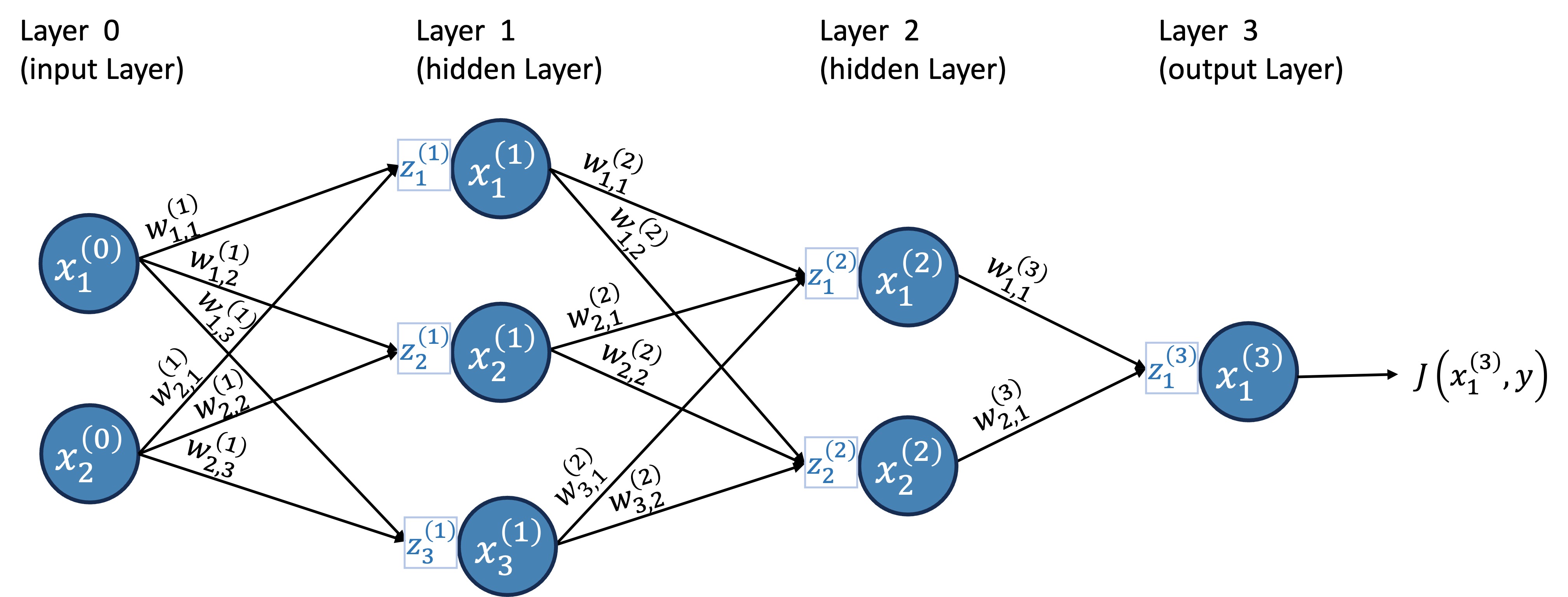
When I started learning about neural networks, I found the standard diagram confusing because it doesn’t explicitly show a crucial component that will be needed later for the backpropagation algorithm. Therefore, for this tutorial, we will explicitly include this component in the diagram, as shown in Figure 2.

Let’s introduce some terminology:
Layers: This neural network has four layers.
- Input layer: the first layer is known as the input layer; it brings the data into the network.
- Output layer: the last layer is known as the output layer; it provides the numerical outputs of the neural network.
- Hidden layers: the layers between the input and output layers are known as the hidden layers; in this case, layers 1 and 2 are hidden layers.
Neurons: the blue circles are the so-called neurons; neurons send a numerical value as a signal for the neurons in the following layer.
- Different layers can have different numbers of neurons.
- The signals neurons in the input layer send are the data.
- The number of neurons in the input layer is the number of attributes in the dataset.
- Activation function: a non-linear function that specifies how neurons process the signals they receive. This function is not explicitly shown in the graph, but it is “inside” the neuron.
Weights: the weights are numerical values (positive or negative) that amplify or reduce the strength of a neuron’s signal to another neuron; they are represented in the graph by the lines;
Receptors: we will call the boxes attached to each neuron the neuron’s receptor, which will collect and aggregate all the signals a neuron receives from other neurons (this is not standard language – this is usually called the “weighted sum” or “pre-activation”).
I’ve always found the terminology very confusing without looking at the equations. For example, when I say that weights amplify or reduce the signal, how exactly does that happen? How exactly do receptors collect and aggregate all the signals? How do neurons process the signals passed by the receptors? Before we go over these in detail, let’s review the notation we are using.
3 Notation
- \((l)\) refers to the layer, and goes from 0 to \(L\), where the \(L\)th layer is the output layer.
- \(n^{(l)}\) is the number of neurons in layer \(l\).
- \(x^{(l)}_{k}\) is the \(k\)th neuron in layer \(l\).
- \(x^{(l)}_{i,k}\) is the value of the \(k\)th neuron in layer \(l\) for the \(i\)th training sample.
- \(z^{(l)}_{k}\) is the receptor of neuron \(x^{(l)}_k\).
- \(z^{(l)}_{i,k}\) is the value of the receptor of neuron \(x^{(l)}_k\) for the \(i\)th training sample.
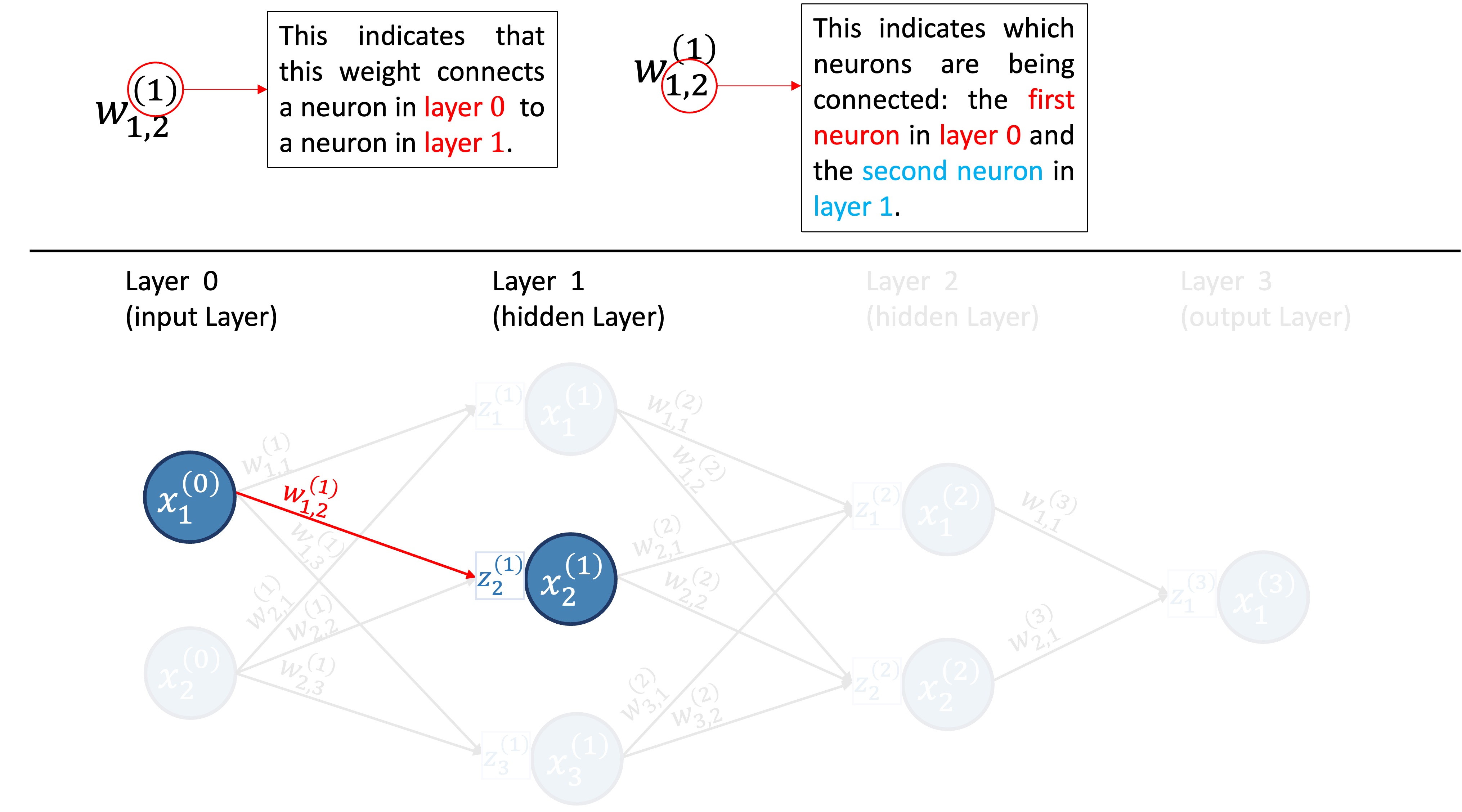
- \(w_{i,j}^{(l)}\) is the weight connecting the \(i\)th neuron in layer \(l-1\) to the \(j\)th neuron in layer \(l\).
- \(b^{(l)}_k\) the bias term added by the receptor of neuron \(k\) in layer \(l\).
Since we have a ton of weights, it is helpful for us to organize them into matrices. We will have one weight matrix per layer (except for layer 0). We will denote the matrices as \({\bf{W}}^{(l)}\). Figure 4 illustrates how the weights are organized into matrices for our example neural network.

The matrix \({\bf{W}}^{(l)}\) contains the weights connecting neurons in layer \(l-1\) to neurons in layer \(l\). It has \(n^{(l-1)}\) rows and \(n^{(l)}\) columns. The \(i\)th row of \({\bf{W}}^{(l)}\) contains all weights “leaving” neuron \(i\) in layer \(l-1\). The \(j\)th column of \({\bf{W}}^{(l)}\) contains all the weights “arriving” in neuron \(j\) in layer \(l\). Figure 5 illustrates these points.
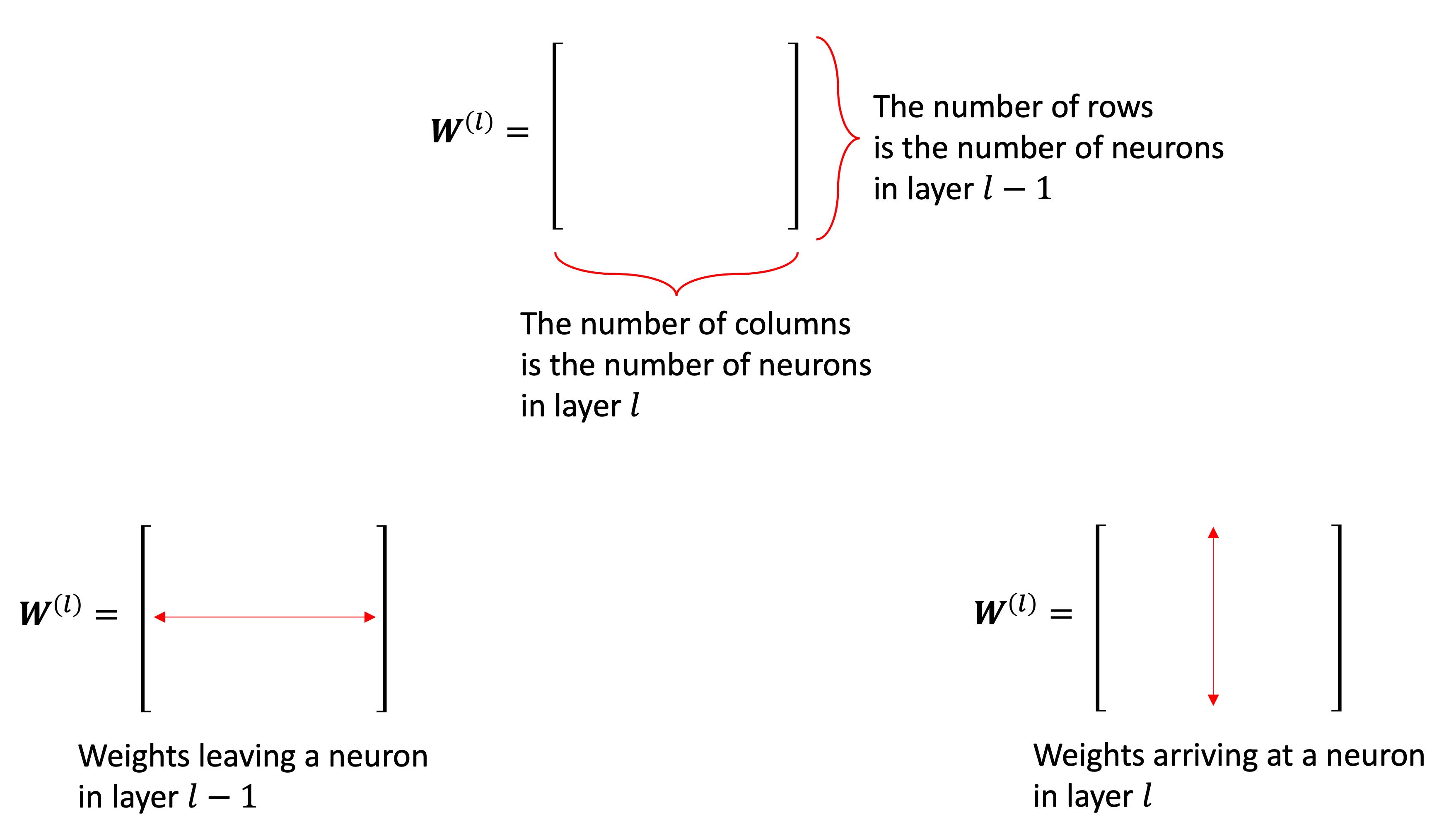
For example, the second row of \({\bf{W}}^{(2)}\) has all the weights leaving neuron 2 from layer 1, as shown in Figure 6; while the second column has all the weights arriving at neuron 2 in layer 2, as illustrated in Figure 7.


Now that we understand the notation, we are ready to introduce the necessary equations.
- Receptors: The value of the \(k\)th receptor in layer \(l\) for the \(i\)th training sample is given by: \[z^{(l)}_{i, k} =\sum_{j=1}^{n^{(l-1)}} w^{(l)}_{j, k}x^{(l-1)}_{i,j} + b^{(l)}_k,\quad l=1,...,L, \quad \text{and} \quad j=1,...,n^{(l)}\]
- Neurons (for the \(i\)th training sample): \[x^{(l)}_{i, k}=a\left(z^{(l)}_{i, k}\right),\quad l=1,...,L, \quad \text{and} \quad j=1,...,n^{(l)}\] where \(a\) is a non-linear function called activation function. We will discuss activation functions in more detail later. For now, we will use \(a(x)=\max\left\{0, x\right\}\).
- Note: for the input layer, \(l=0\), \(x^{(0)}_j\) is just the feature \(j\) of the input vector.
Okay, I agree; the notation is heavy. We have a lot of things to keep track of, such as layers, receptors, neurons, and weights, so we need a lot of symbols and indices. For this reason, I encourage the reader to go back to Figure 2, pick a neuron in a hidden layer, and write down the equations for that neuron while identifying the elements being used in the diagram.
Example 1 For us to go through an example of the feedforward part of the neural network, let us get some synthetic data with two features as well as define some values for the weights.
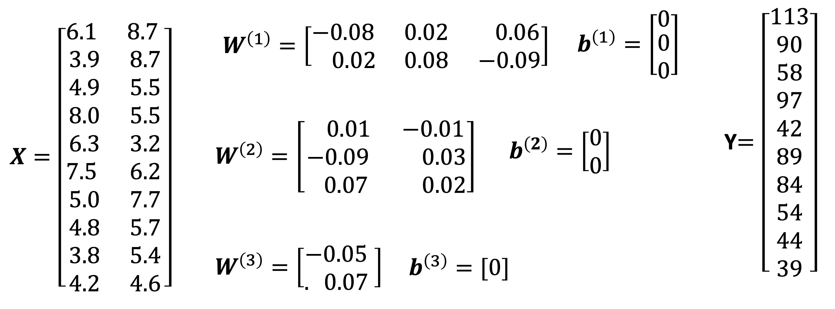
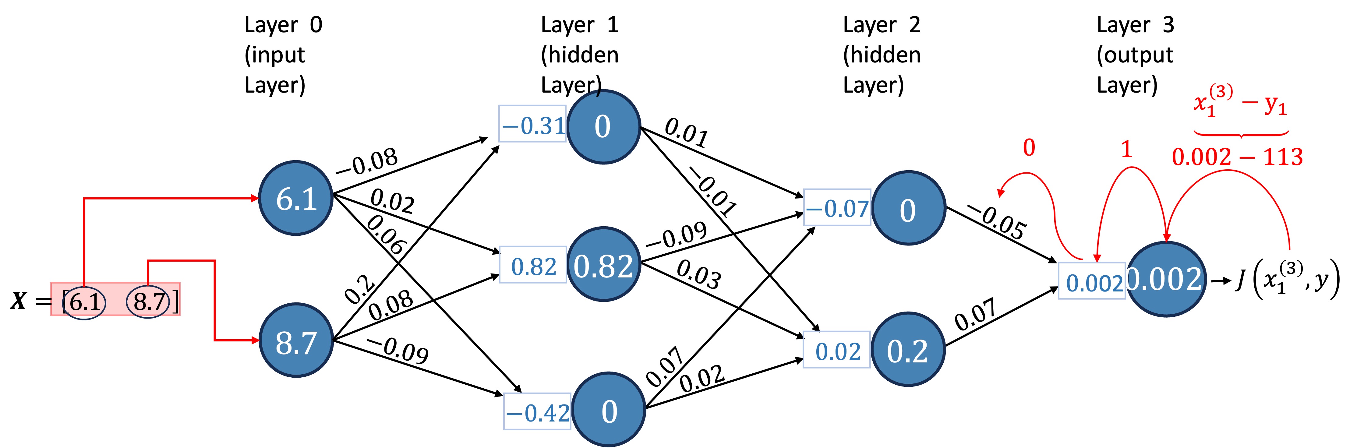
Now, we can calculate the forward pass of the neural network. Let’s do it for the first row in our data, i.e., for the input vector \(x=(6.1, 8.7)\).
Receptors in Layer 1: \[z^{(1)}_1 =\sum_{i=1}^{2} w^{(1)}_{i, 1}x^{(0)}_i + b^{(1)}_1 = -0.314\] \[z^{(1)}_2 =\sum_{i=1}^{2} w^{(1)}_{i, 2}x^{(0)}_i + b^{(1)}_2 = 0.818\] \[z^{(1)}_3 =\sum_{i=1}^{2} w^{(1)}_{i, 3}x^{(0)}_i + b^{(1)}_3 = -0.417\]
Receptors in Layer 2: \[z^{(2)}_1 =\sum_{i=1}^{3} w^{(2)}_{i, 1}x^{(1)}_i + b^{(2)}_1 = -0.07362\] \[z^{(2)}_2 =\sum_{i=1}^{3} w^{(2)}_{i, 2}x^{(1)}_i + b^{(2)}_2 = 0.02454\]
Receptor in Layer 3: \[z^{(3)}_1 =\sum_{i=1}^{2} w^{(3)}_{i, 1}x^{(1)}_i + b^{(3)}_1 = 0.0017178\]
Neurons in Layer 1: \[x^{(1)}_1 = \max\left\{0, z^{(1)}_1\right\} = 0\ \ \ \ \ \ \textcolor{white}{\sum_{i=1}^{2}}\] \[x^{(1)}_2 = \max\left\{0, z^{(1)}_2\right\} = 0.818 \textcolor{white}{\sum_{i=1}^{2}}\] \[x^{(1)}_3 = \max\left\{0, z^{(1)}_3\right\} = 0\ \ \ \ \ \ \textcolor{white}{\sum_{i=1}^{2}}\]
Neurons in Layer 2: \[x^{(2)}_1 = \max\left\{0, z^{(2)}_1\right\} = 0\ \ \ \ \ \ \ \ \ \ \textcolor{white}{\sum_{i=1}^{2}}\] \[x^{(2)}_2 = \max\left\{0, z^{(2)}_2\right\} = 0.02454 \textcolor{white}{\sum_{i=1}^{2}}\]
Neuron in Layer 3: \[x^{(3)}_1 = z^{(3)}_1 = 0.0017178\]
Let’s now visualize this result in the diagram. We will use two decimal places due to space constraints.

Congratulations! You have completed the forward pass of the neural network.
I’ll just note here that the activation function used in the output layer usually changes according to the problem. For example, for regression problems, a common choice is the identity function \(f(z) = z\). If we used \(f(z) = \max\left\{0, z\right\}\), we would never be able to predict a negative value, an undesirable property.
3.1 Matrix Notation
To implement a Neural Network in Python from scratch, we will need to use the highly optimized Numpy’s vectorization; so, let’s introduce the matrix notation here. The matrix notation also has the advantage of simplifying the steps. Note that everything is almost exactly the same; the only difference is that, with the matrix notation, we will be considering the entire dataset.
We will denote matrices with capital bold letters (e.g., \(\bf{X}\), \({\bf{W}}^{(1)}\)), vectors as lowercase bold letters (e.g., \({\bf{x}}_1\)). Also, vectors are always column vectors (multiple rows, one column). Here are the equations in matrix format:
Receptors: \[ {\bf{Z}}^{(l)} = {\mathbf{X}^{(l-1)}} \mathbf{W}^{(l)} + \mathbf{1}_n\left(\mathbf{b}^{(l)}\right)^\top \tag{1}\] where \(\mathbf{1}_n\) is a column vector of ones with \(n\) rows and \((\cdot)^\top\) denotes transpose. The operation \(\mathbf{1}_n\left(\mathbf{b}^{(l)}\right)^\top\) is Numpy’s broadcast. This operation broadcasts the bias vector across all \(n\) samples (mathematically represented here as an outer product with a vector of ones).
Neurons: \[ {\bf{X}}^{(l)} = a\left({\bf{Z}}^{(l)}\right) \tag{2}\] where \(a\left({\bf{Z}}^{(l)}\right)\) means we apply the activation function \(a\) to every single element of \({\bf{Z}}^{(l)}\).
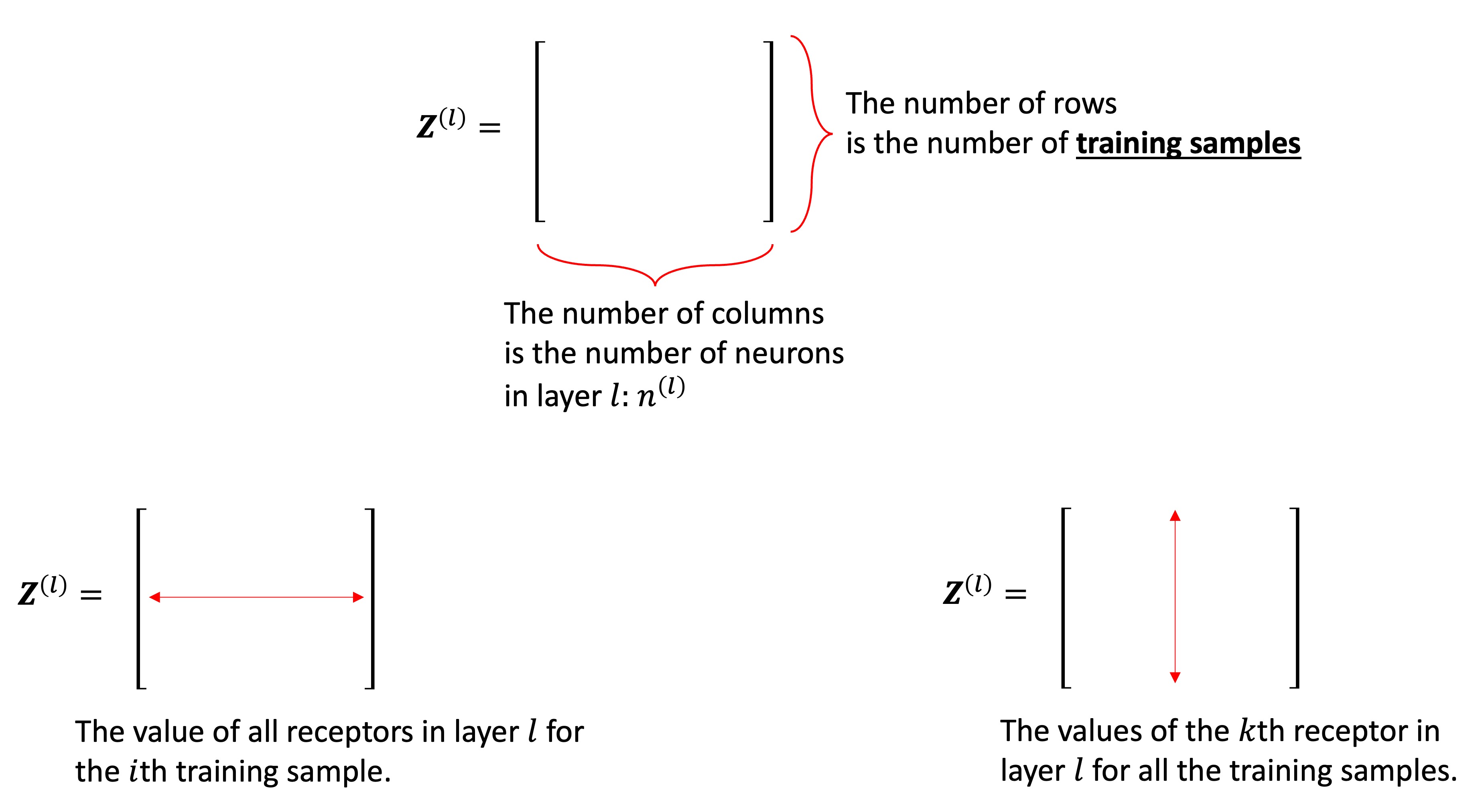
The notation becomes much simpler, doesn’t it? Let’s take a closer look at \({\bf{Z}}^{(l)}\) in Figure 10 .
Now, let’s go through Example 1 again, but this time, we will use matrix notation.
Example 2 We will use the same data and weights as before, as shown in Figure 8. The forward pass involves calculating the values of the receptors and neurons for each layer of the network and each input vector. We will start by calculating \({\bf{Z}}^{(1)}\), \({\bf{X}}^{(1)}\), \({\bf{Z}}^{(2)}\), \({\bf{X}}^{(2)}\), \({\bf{Z}}^{(3)}\), and \({\bf{X}}^{(3)}\) for all input vectors. We will first do it mathematically, then we will implement it in Python.
- We start by calculating \({\bf{Z}}^{(1)}\) and \({\bf{X}}^{(1)}\):

- Using the results from the first layer, we can calculate \({\bf{Z}}^{(2)}\) and \({\bf{X}}^{(2)}\):

- Using the results from the second layer, we can calculate \({\bf{Z}}^{(3)}\) and \({\bf{X}}^{(3)}\):

Now that we have the results for all layers and all input vectors, we can implement the forward pass of the neural network in Python. We start by generating the data and initializing the weights.
Great, this matches the data and weights in Figure 8.
Next, we can calculate \({\bf{Z}}^{(1)}\), \({\bf{Z}}^{(2)}\), and \({\bf{Z}}^{(3)}\) and \({\bf{X}}^{(1)}\), \({\bf{X}}^{(2)}\), and \({\bf{X}}^{(3)}\)
NoteYour turn!
Exercise 1 (Forward Pass) Implement the forward pass for the entire dataset using matrix multiplication. Calculate Z1, X1, Z2, X2, Z3, and X3.
Remember the formulas: \[ {\bf{Z}}^{(l)} = {\mathbf{X}^{(l-1)}} \mathbf{W}^{(l)} + \mathbf{1}_n\left(\mathbf{b}^{(l)}\right)^\top \] \[ {\bf{X}}^{(l)} = a\left({\bf{Z}}^{(l)}\right) \]
In Python/Numpy:
- Matrix multiplication:
@ - ReLU activation:
np.fmax(0, Z) - Identity activation:
X = Z
Z1 = X @ W1 + b1
X1 = np.fmax(0, Z1)

Z2 = X1 @ W2 + b2
X2 = np.fmax(0, Z2)

Z3 = X2 @ W3 + b3
X3 = Z3 # Identity activation function for output layer

# Printing the results
print(f'Z1: {Z1}\n\nX1: {X1}\n\nZ2: {Z2}\n\nX2: {X2}\n\nZ3: {Z3}\n\nX3: {X3}')
Z1 = X @ W1 + b1
X1 = np.fmax(0, Z1)

Z2 = X1 @ W2 + b2
X2 = np.fmax(0, Z2)

Z3 = X2 @ W3 + b3
X3 = Z3 # Identity activation function for output layer

# Printing the results
print(f'Z1: {Z1}\n\nX1: {X1}\n\nZ2: {Z2}\n\nX2: {X2}\n\nZ3: {Z3}\n\nX3: {X3}')
We successfully calculated the values of the receptors and neurons for all layers and input vectors using NumPy’s vectorization.
By now, you should have a clear understanding of how the forward pass operates. If not, do not move to the next section. Practice a little more with the information above. There is a lot going on; the notation is heavy, and the matrix notation is a bit confusing at first. Once you are comfortable with the forward pass, we can move on to the backpropagation algorithm. Backpropagation is the algorithm we use to train the neural network. Without training, the output of the neural network is meaningless.
4 Backpropagation
Backpropagation is a critical algorithm employed in the training of neural networks. Its foundation lies in the chain rule of calculus, which allows us to compute how changes in the weights affect the overall performance of the network. The algorithm is named after its distinctive process of error propagation. The algorithm transmits the error from the output layer back through the various layers of the network all the way to the input layer. During this backward pass, the algorithm essentially assesses how much each weight contributed to the overall error, allowing for precise adjustments to be made. By updating these weights using the calculated gradients, the network can gradually improve its predictions and performance.
4.1 Measuring the error: the cost function
Before we delve into the backpropagation algorithm, we need to define a cost function. The cost function quantifies how inaccurate the network’s predictions are. The goal of the training process is to minimize this cost function.
For example, for regression, a commonly used cost function is:
\[ J(\mathbf{w}|\mathbf{X}, \mathbf{y}) = \frac{1}{2n}\sum_{i=1}^{n} \left(\hat{y}_i - y_i\right)^2 \tag{3}\]
where \(\hat{y}_i\) is the predicted value for the \(i\)th sample, \(y_i\) is the true value, and \(n\) is the number of samples. Note that the cost function depends on the weights \(\mathbf{w}\), the input data \(\mathbf{X}\), and the true values \(\mathbf{y}\). But the input data and true values are fixed (it is the data we have); we can only change the weights. Classification problems have different cost functions, such as the cross-entropy loss (let’s not worry about this for now).
4.1.1 Minimizing the cost function
To minimize the cost function, we will use gradient descent. Gradient descent is an optimization algorithm that iteratively adjusts the parameters (in our case, the weights) in the direction that reduces the cost function. The key idea is to start with random weights and then adjust them iteratively based on the gradient of the cost function: \[ w_{ij}^{(l)} := w_{ij}^{(l)} - \eta \frac{\partial}{\partial w_{ij}^{(l)}}J(\mathbf{w}|\mathbf{X}, \mathbf{y}) \]
where \(\eta\) is the learning rate, a small positive number that controls the size of each update .
To use this algorithm, we need to compute the derivative (gradient) of the cost function with respect to each weight in the network. This is where backpropagation comes into play.
4.2 The backpropagation algorithm
The entire idea of backpropagation is to calculate the gradient of the cost function with respect to the weights. To do this, we need to pass through the elements of the network in reverse order. We will start by calculating the gradient of the cost function with respect to the neurons in the output layer. Then, we will calculate the gradient of the cost function with respect to the receptors in the output layer. Finally, we will calculate the gradient of the cost function with respect to the weights.
In this section, we will illustrate the backpropagation algorithm using our example Neural Network. Recall the specific settings for this example:
- The activation function for the hidden layers is the ReLU, defined as \(a(x) = \max\{0, x\}\).
- The activation function for the output layer is the identity function, \(a^{(L)}(x) = x\).
- The cost function is the Mean Squared Error, as given by Equation 3.
Additionally, while the bias terms are omitted from our diagrams for clarity, they must also be included in the calculations. You can conceptualize the bias as an additional weight connected to a neuron with a constant value of 1. Naturally, these choices influence the derivative calculations. We will first focus on understanding the process with these specific settings before introducing the general backpropagation formula.
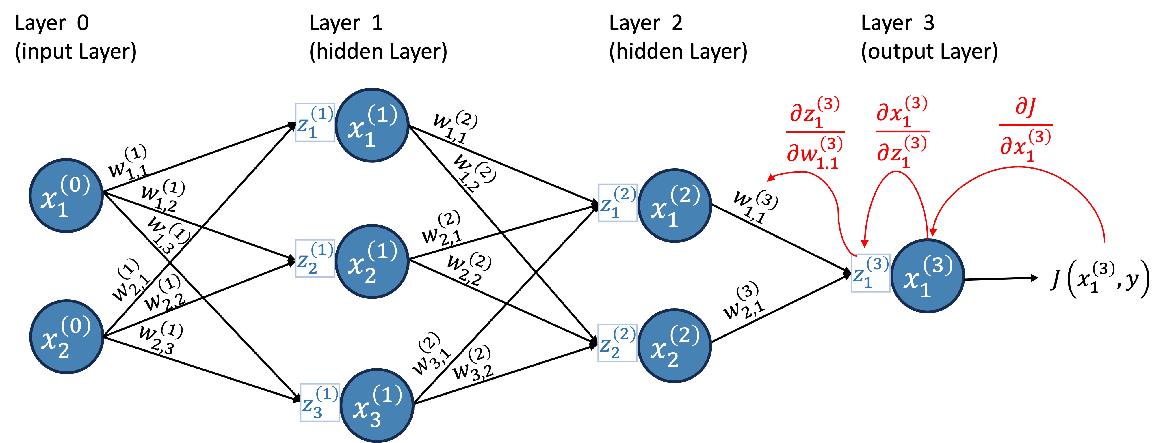
To visualize the backpropagation step-by-step, let’s update our neural network diagram with the cost function, as shown in Figure 14.
For now, let’s do this for a single input vector (as if our data matrix \(X\) had only one row). Remember, the weights are the only thing we can change; the data and true values are fixed. So, we want to calculate the gradient of the cost function with respect to the weights. Let’s start with the output layer and calculate the derivative of \(w_{1,1}^{(3)}\).
4.2.1 Layer 3: Output layer
We will calculate this derivative using the chain rule:
First, we calculate the derivative of the cost function with respect to the neuron \(x^{(3)}_1\): \(\frac{\partial J}{\partial x^{(3)}_1}\).
Then, we calculate the derivative of the neuron \(x^{(3)}_1\) with respect to the receptor \(z^{(3)}_1\): \(\frac{\partial x^{(3)}_1}{\partial z^{(3)}_1}\).
(Note that since \(x = a(z)\), this is simply the derivative of the activation function, \(a'(z)\).)Finally, we calculate the derivative of the receptor \(z^{(3)}_1\) with respect to the weight \(w_{1,1}^{(3)}\): \(\frac{\partial z^{(3)}_1}{\partial w_{1,1}^{(3)}}\).
(Note that since \(z^{(3)}_1 = \sum_{i=1}^{2} w^{(3)}_{i, 1}x^{(2)}_i\), this is simply \(x^{(2)}_1\).)
Then, we combine these using the chain rule: \[ \frac{\partial J}{\partial w_{1,1}^{(3)}} = \frac{\partial J}{\partial x^{(3)}_1}\frac{\partial x^{(3)}_1}{\partial z^{(3)}_1}\frac{\partial z^{(3)}_1}{\partial w_{1,1}^{(3)}} \tag{4}\]
Figure 15 illustrates the calculation of the derivative of \(w_{1,1}^{(3)}\).
Tip 1: Backprop Derivatives - it’s always the same!
Admittedly, this looks complicated at first, with lots of terms, and it gets worse when the path becomes longer. The notation becomes heavier. But don’t let the heavy notation scare you off. Each of these partial derivatives is straightforward to calculate. In fact, there are three derivatives that will keep showing up throughout the backpropagation algorithm, if you keep those three in mind, everything translates easily (once you get the hang of it):
- The first one that will appear frequently is the derivative of the neuron \(x^{(l)}_j\) with respect to the receptor \(z^{(l)}_j\): \[\frac{\partial x^{(l)}_j}{\partial z^{(l)}_j}\] This is just the derivative of the activation function: \(a^\prime\left(z^{(l)}_j\right)\). Note the layer is the same for both \(x\) and \(z\).
- For example, if we use the ReLU activation function, this derivative is: \[ \frac{\partial x^{(l)}_j}{\partial z^{(l)}_j} = a^\prime\left(z^{(l)}_j\right) = \begin{cases} 1 & \text{if } z^{(l)}_j > 0 \\ 0 & \text{if } z^{(l)}_j \leq 0 \end{cases} \] every time you see \(\frac{\partial x^{(l)}_j}{\partial z^{(l)}_j}\), you can replace it with the expression above.
- The second one that will appear frequently is the derivative of the receptor \(z^{(l)}_j\) with respect to the weight \(w_{i,j}^{(l)}\): \[\frac{\partial z^{(l)}_j}{\partial w_{i,j}^{(l)}}\] Well, \(z^{(l)}_j\) is just a linear combination of the weights and neurons from the previous layer, \(z^{(l)}_j = \sum_{k=1}^{n^{(l-1)}} w^{(l)}_{k, j}x^{(l-1)}_k + b^{(l)}_j\). So, the derivative of \(z^{(l)}_j\) with respect to \(w_{i,j}^{(l)}\), is just the value of the neuron \(x^{(l-1)}_i\) from the previous layer.
- So, every time you see \(\frac{\partial z^{(l)}_j}{\partial w_{i,j}^{(l)}}\), you can replace it with \(x^{(l-1)}_i\). (Note the layer of \(z\) is \(l\), while the layer of \(x\) is \(l-1\).
- The third one that will appear is the derivative of the receptor in layer \(l\) with respect to the neuron in layer \(l-1\): \(\frac{\partial z^{(l)}_k}{\partial x^{(l-1)}_j}\). This is just the weight \(w_{j,k}^{(l)}\) connecting neuron \(j\) in layer \(l-1\) to neuron \(k\) in layer \(l\). So, every time you see \(\frac{\partial z^{(l)}_k}{\partial x^{(l-1)}_j}\), you can replace it with \(w_{j,k}^{(l)}\). (Note the layer of \(z\) is \(l\), while the layer of \(x\) is \(l-1\).)
With that in mind, let’s calculate each of the three derivatives in Equation 4:
First, \(\frac{\partial J}{\partial x^{(3)}_1}\): \[\frac{\partial J}{\partial x^{(3)}_1} = \frac{\partial}{\partial x^{(3)}_1}\left[\frac{1}{2}\left(x^{(3)}_1 - y_1\right)^2\right] = x^{(3)}_1 - y_1 \tag{5}\]
Next, \(\frac{\partial x^{(3)}_1}{\partial z^{(3)}_1}\): \[\frac{\partial x^{(3)}_1}{\partial z^{(3)}_1} = \frac{\partial}{\partial z^{(3)}_1}z^{(3)}_1 = 1 \tag{6}\] (Remember we are using the identity function as the activation function for the last layer since this is a regression problem, i.e., \(x^{(3)}_1=z^{(3)}_1\).)
Finally, as discussed in the last point of Tip 1: \[\frac{\partial z^{(3)}_1}{\partial w_{1,1}^{(3)}} = \frac{\partial}{\partial w_{1,1}^{(3)}}\left[\sum_{i=1}^{2} w^{(3)}_{i, 1}x^{(2)}_i\right] = x^{(2)}_1\]
Note the presence of \(x^{(2)}_1\) and \(x^{(3)}_1\) in the derivatives. These are the values obtained in the forward pass.
Therefore, the derivative of \(\frac{\partial J}{\partial w_{1,1}^{(3)}}\) is: \[ \frac{\partial J}{\partial w_{1,1}^{(3)}} = (x^{(3)}_1 - y_1) \times 1 \times x^{(2)}_1 \tag{7}\] which, in this case, \[ \frac{\partial J}{\partial w_{1,1}^{(3)}} = (0.0017178 - 113) \times 1 \times 0 = 0 \]
The diagram Figure 16 illustrates the values of the derivatives for the example we have been working on.
Z3, X3, and X2 in Exercise 1.)
Similarly, we can calculate the derivative of \(w_{2,1}^{(3)}\). But you don’t learn by me doing it for you; you learn by doing it yourself, see Exercise 2 below. As a hint, Figure 17 illustrates the calculation of the derivative of \(w_{2,1}^{(3)}\).
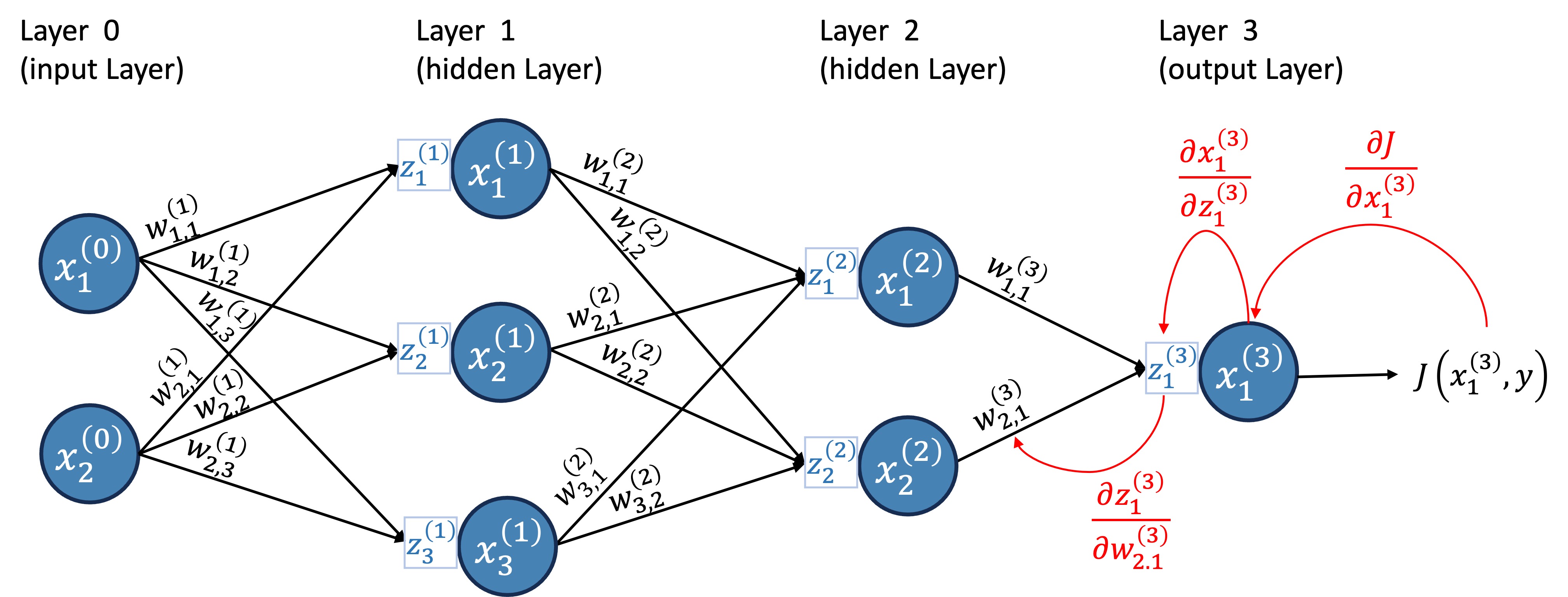
NoteYour turn!
Exercise 2 (Derivative of the cost function) Calculate the derivative of the cost function with respect to \(w_{2,1}^{(3)}\) for the first data point. Store the result in a variable named dj_dw3_21.
Recall the chain rule: \[ \frac{\partial J}{\partial w_{2,1}^{(3)}} = \frac{\partial J}{\partial x^{(3)}_1}\frac{\partial x^{(3)}_1}{\partial z^{(3)}_1}\frac{\partial z^{(3)}_1}{\partial w_{2,1}^{(3)}} \] And the values: \[ \frac{\partial J}{\partial x^{(3)}_1} = (x^{(3)}_1 - y_1) \] \[ \frac{\partial x^{(3)}_1}{\partial z^{(3)}_1} = 1 \] \[ \frac{\partial z^{(3)}_1}{\partial w_{2,1}^{(3)}} = x^{(2)}_2 \]
Therefore, \[ \frac{\partial J}{\partial w_{2,1}^{(3)}} = (0.0017178 - 113) \times 1 \times 0.02454 \approx −2.77 \]
# Derivative of Cost w.r.t prediction
dJ_dx3 = X3[0, 0] - Y[0]

# Derivative of prediction w.r.t receptor (Identity activation)
dx3_dz3 = 1

# Derivative of receptor w.r.t weight
dz3_dw3_21 = X2[0, 1] # 2nd neuron (index 1) of layer 2

dj_dw3_21 = dJ_dx3 * dx3_dz3 * dz3_dw3_21
print(dj_dw3_21)
# Derivative of Cost w.r.t prediction
dJ_dx3 = X3[0, 0] - Y[0]

# Derivative of prediction w.r.t receptor (Identity activation)
dx3_dz3 = 1

# Derivative of receptor w.r.t weight
dz3_dw3_21 = X2[0, 1] # 2nd neuron (index 1) of layer 2

dj_dw3_21 = dJ_dx3 * dx3_dz3 * dz3_dw3_21
print(dj_dw3_21)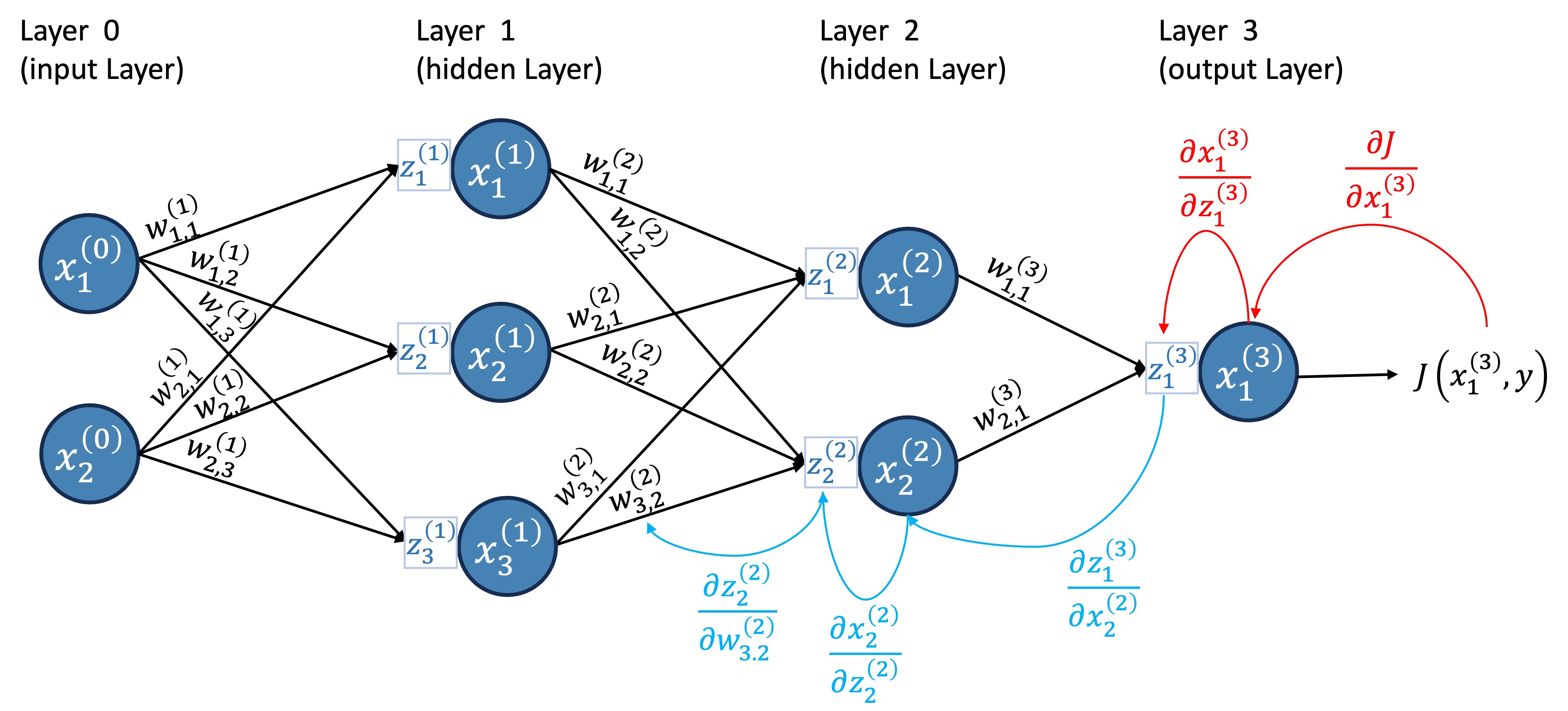
 Chain rule for the derivative of
 4.2.4 General Formula for Backpropagation
Let’s now summarize the backpropagation algorithm, and then attempt to write it in a more general form.
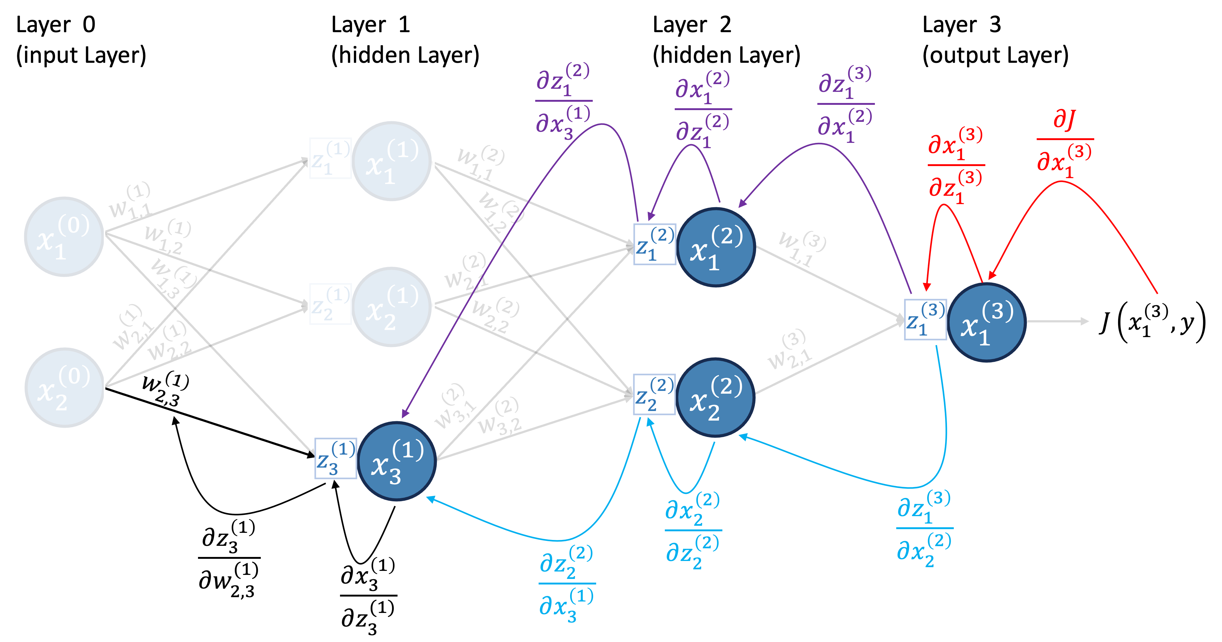
A key element of the paths we constructed for the derivatives in backpropagation were the receptors. Once we got the derivative of the cost function with respect to the receptor of a neuron, we could easily get the derivative with respect to any weight connected to that neuron, and we could also move backwards to the previous layer:
Note from Figure 15, Figure 17, Figure 18, and Figure 19 that to calculate the derivative of the cost function with respect to any weight \(w_{j,k}^{(l)}\), we always started by calculating the derivative of the cost function with respect to the respective receptor of that weight (note how the last arrow is always from a receptor to a weight);
Also, note from Figure 18 and Figure 19, that every time we wanted to switch layer, we always went from the receptors of a layer to a neuron from the previous layer, and finally reached the receptor of the previous layer;
Therefore, a key term in backpropagation is the derivative of the cost function with respect to the receptor of a neuron: \(\frac{\partial J}{\partial z^{(l)}_{k}}\). To simplify the notation, let’s denote this term as \(\delta^{(l)}_{k}\) (i.e., \(\delta^{(l)}_{k} = \frac{\partial J}{\partial z^{(l)}_{k}}\)) (this is a common notation is DL literature).
All expressions below are written for a single input vector (one training sample). For a dataset with \(n\) samples, compute these quantities for each sample and then average across samples.
This term, \(\delta^{(l)}_{k} = \frac{\partial J}{\partial z^{(l)}_{k}}\), essentially captures how much the cost function changes when we make a small change to the receptor of neuron \(k\) in layer \(l\).
Next, say that you want to calculate \(\delta^{(l)}_{k}\) for any hidden layer \(l\) and neuron \(k\). Since we are going backwards, we start from the output layer:
For the output layer (\(l=L\)), we can calculate \(\delta^{(L)}_{k}\) as: \[ \delta^{(L)}_{k} = \frac{\partial J}{\partial x^{(L)}_{k}} \frac{\partial x^{(L)}_{k}}{\partial z^{(L)}_{k}} \tag{8}\] where \(\frac{\partial J}{\partial x^{(L)}_{k}}\) depends on the cost function we are using (for example, for MSE, we have Equation 5), and \(\frac{\partial x^{(L)}_{k}}{\partial z^{(L)}_{k}}\) is just the derivative of the activation function used in the output layer (for example, for the identity function, we have Equation 6).
For hidden layers (\(l < L\)), we can calculate \(\delta^{(l)}_{k}\) as: but remember we already have \(\delta^{(l+1)}_{m}\) for all neurons \(m\) from layer \((l+1)\) (see Figure 19).
Finally, once we have \(\delta^{(l)}_{k}\), we can calculate the derivative of the cost function with respect to any weight \(w_{i,k}^{(l)}\) as: \[ \frac{\partial J}{\partial w_{i,k}^{(l)}} = \delta^{(l)}_{k} \times x^{(l-1)}_{i} \tag{10}\] where \(x^{(l-1)}_{i}\) is the output of neuron \(i\) from the previous layer \((l-1)\).
Similarly, for the bias term \(b^{(l)}_k\) we have: \[ \frac{\partial J}{\partial b^{(l)}_{k}} = \delta^{(l)}_{k} \tag{11}\]
We now have everything we need to create our feedforward neural network class and implement the training algorithm using backpropagation!
5 Implementation with NumPy
In this section, we will implement the forward and backward propagation algorithms for training a simple feedforward neural network. We start by doing it from scratch using just Numpy, where we have to implement all the steps ourselves.
To implement our Neural Network, we will create a Python class named NN.
Before writing any code, let’s understand how this class will operate and what it needs to be initialized. The NN class will be initialized with four arguments:
layers_dims: A list of integers representing the number of neurons in each layer. For example,layers_dims=[2, 3, 1]means:- Layer 0 (Input): 2 neurons
- Layer 1 (Hidden): 3 neurons
- Layer 2 (Output): 1 neuron
activation_hidden: This defines the activation functions for the hidden layers of the network (layers \(1\) to \(L-2\)). The activation will be specified as a dictionary of the form:
{
    'activation': activation_function,
    'derivative': derivative_activation_function
}- If a single dictionary is passed, it will be used for all layers (except the input layer, which is just the data itself) and the output layer.
- A list of dictionaries, specifying a different activation function for each layer.
activation_output: Similar toactivation_hidden, but specifically for the output layer (layer \(L-1\)).loss_function: A dictionary containing the loss function and its derivative
{
    'loss': loss_function,
    'derivative': derivative_loss_function
}
The network relies on knowing how to calculate the activations and loss functions, as well as their derivatives. This information will be passed as dictionaries. In the following exercises, you will implement the dictionaries for the activation functions and the loss function.
5.1 Activation functions
Let’s start by defining the activation function for the hidden layers.
NoteYour turn!
Exercise 5 (Implement ReLU) For the hidden layers, we will use the ReLU (Rectified Linear Unit) function. Remember, the ReLU function is defined as: \[ a(z) = \max(0, z) \]
Do you remember the derivative of the ReLU function?
- Take a look at the function
np.maximum(it’s efficient and handles arrays automatically). - The derivative is 1 where
z > 0, and 0 otherwise. You can use boolean indexing ornp.where.
def relu(z):
    """
    Computes the ReLU activation function.
    Args:
        z (numpy.ndarray): Input array.
    Returns:
        numpy.ndarray: Output after applying ReLU.
    """
    return np.maximum(0, z)

def relu_derivative(z):
    """
    Computes the derivative of the ReLU activation function.
    Args:
        z (numpy.ndarray): Input array.
    Returns:
        numpy.ndarray: Output after applying the derivative of ReLU.
    """
    return (z > 0).astype(float)

activation_relu_dict = {
    'activation': relu,
    'derivative': relu_derivative
    }
Next, we will define the activation function for the output layer.
NoteYour turn!
Exercise 6 (Activation for output layer) Since we are building a regression network, the output layer will use the Identity function: \[a(z) = z\]
Implement identity(z) and identity_derivative(z).
- Function: simply return \(z\).
- Derivative: \(a'(z) = 1\). See the function
np.ones_liketo ensure you return an array of 1s with the same shape as the input.
def identity(z):
    """
    Computes the identity activation function.
    Args:
        z (numpy.ndarray): Input array.
    Returns:
        numpy.ndarray: Output after applying identity activation.
    """
    return z

def identity_derivative(z):
    """
    Computes the derivative of the identity activation function.
    Args:
        z (numpy.ndarray): Input array.
    Returns:
        numpy.ndarray: Output after applying the derivative of the identity activation.
    """
    return np.ones_like(z)

activation_output_dict = {
    'activation': identity,
    'derivative': identity_derivative
    }
5.2 Loss Function
Finally, we will define the loss function. The loss function we will use is the Mean Squared Error (MSE) loss: \[ J(X, Y) = \frac{1}{2n} \sum_{i=1}^{n} (\hat{y}_i - y_i)^2 \]
NoteYour turn!
Exercise 7 (Mean Squared Error Loss) Implement MSE(y_hat, y) and MSE_derivative(y_hat, y), where:
y_hat: the network’s predicted values.y: the true values.
- MSE: you might want to use
np.meanto compute the average. - Derivative: \(J^\prime(\hat{y}_i) = \frac{1}{n}(\hat{y}_i - y)\).
- Remember that
y.shape[0]gives the number of samples (\(n\)).
- Remember that
def MSE(a, Y):
    """
    Computes the Mean Squared Error loss.
    Args:
        y_hat (numpy.ndarray): Predicted values.
        Y (numpy.ndarray): True values.
    Returns:
        float: Mean Squared Error loss.
    """
    return np.mean((a - Y) ** 2)/2

def MSE_derivative(a, Y):
    """
    Computes the derivative of Mean Squared Error loss with respect to predictions.
    Args:
        y_hat (numpy.ndarray): Predicted values.
        Y (numpy.ndarray): Response variable.
    Returns:
        numpy.ndarray: Derivative of the MSE loss.
    """
    return (a - Y) / Y.shape[0]

loss_dict = {
    'loss': MSE,
    'derivative': MSE_derivative
    }
5.3 Creating the Neural Network Class: NN
Now we will define the NN class. We have written the skeleton of the class for you. For example, the __init__ boilerplate is already provided with comments – please read and understand it.
class NN:

    def __init__(self, layers_dims, activation_hidden, activation_output, loss_function, seed=None):
        """
        Initializes the neural network with random weights and biases.

        Args:
            layers_dims (list): Dimensions of layers including input layer.
                                Example: [2, 3, 1] implies 2 input nodes, 3 hidden nodes, and 1 output node.
            activation_hidden (dict or list of dict): Activation function(s) for the hidden layers (Layers 1 to L-2).
                                If a single dict is provided, it is applied to all hidden layers.
                                If a list is provided, it must specify the activation for each hidden layer individually.
                                Example: {'activation': relu, 'derivative': relu_derivative}
            activation_output (dict): Activation function for the output layer (Layer L-1).
                                Example: {'activation': linear, 'derivative': linear_derivative}
            loss_function (dict): Cost function and its derivative.
                                Example: {'loss': mse, 'derivative': mse_derivative}
        """

        # The number of layers in the network
        self.L = len(layers_dims)

        self.loss_function = loss_function

        # Dictionary to hold weights and biases
        self.params = {}

        # Processing the activation functions:
        # 1. Input layer (Layer 0) is always Identity
        self.a = [lambda x: x]

        # 2. Hidden layers (Layers 1 to L-2)
        if isinstance(activation_hidden, list):
            self.a.extend(activation_hidden)
        else:
            # Replicate dict for all hidden layers (Total - Input - Output)
            self.a.extend([activation_hidden] * (self.L - 2))

        # 3. Output layer (Layer L-1)
        self.a.append(activation_output)

        # Initialize parameters
        rng = np.random.default_rng(seed=seed)
        self.initialize_parameters(layers_dims, rng)

    def initialize_parameters(self, layers_dims, rng):
        """
        Initializes weights and biases.
        self.params should contain keys 'W1', 'b1', ...
        Args:
            layers_dims (list): List of layer dimensions.
            rng (np.random.Generator): random number generator for reproducibility.
        """
        pass

    def forward_pass(self, X, training=False):
        """
        Performs a forward pass through the network.
        """
        pass

    def backward_pass(self, X, Y, coef):
        """
        Computes gradients using backpropagation.
        Args:
            X (numpy.ndarray): Input data, shape n x p, where n is the number of training samples and p the number of attributes.
            Y (numpy.ndarray): True labels, shape n x m, where m is the number of output neurons.
            coef (dict): Intermediate values from forward pass.
                            Example: {'x0': np.array([[1, 2], [2, 3]]), 'z1': ...}
        Returns:
            dict: Gradients of loss with respect to weights and biases.
        """
        pass

    def train(self, X, Y, n_it, learning_rate=0.01, verbose=True):
        """
        Trains the neural network using gradient descent.

        Args:
            X (numpy.ndarray): Input data.
            Y (numpy.ndarray): True labels.
            n_it (int): Number of training iterations.
            learning_rate (float): Step size for gradient descent. Defaults to 0.01.
        """
        pass
Your task is to fill in the missing parts, starting with the initialization of the network parameters (weights and biases).
5.3.1 Parameter Initialization
The weights and biases of the network need to be initialized before training. We will initialize the weights with tiny random values drawn from a normal distribution (\(N(0, \sigma^2)\), with a small value for \(\sigma\)). Biases will be initialized to zero.
NoteYour turn!
Exercise 8 (Parameter Initialization) Implement the loop to initialize self.params. Here are the details:
Iterate from Layer 1 up to Layer L-1. (Layer 0 has no weights “arriving” at it).
Initialize weights (\(\mathbf{W}^{(l)}\)) with values drawn from a normal distribution with
scale=0.001.- You can generate values from a normal distribution with the function
rng.normal.
- You can generate values from a normal distribution with the function
Initialize biases (\(\mathbf{b}^{(l)}\)) with zeros (see
np.zeros).Store the weights and biases in
self.paramsdictionary, usingkeys like
W1,b1,W2,b2, etc.
Remember, the weights connect every neuron from the previous layer to every neuron in the current layer.
- Loop range: range(1, self.L)
- Previous layer size: layers_dims[l-1]
- Current layer size: layers_dims[l]
def initialize_parameters(self, layers_dims, rng):
    for l in range(1, self.L):
        self.params[f'W{l}'] = rng.normal(scale=0.001, size=(layers_dims[l - 1], layers_dims[l]))
        self.params[f'b{l}'] = np.zeros((1, layers_dims[l]))

NN.initialize_parameters = initialize_parameters
def initialize_parameters(self, layers_dims, rng):
    for l in range(1, self.L):
        self.params[f'W{l}'] = rng.normal(scale=0.001, size=(layers_dims[l - 1], layers_dims[l]))
        self.params[f'b{l}'] = np.zeros((1, layers_dims[l]))

NN.initialize_parameters = initialize_parameters
5.3.2 Forward Pass
Now we implement the forward_pass method. This method is responsible for flowing the data from the input layer (\(x^{(0)}\)) through the hidden layers to the output layer (\(x^{(L-1)}\)).
An important implementation note is that to train the neural network with backpropagation, we will need the outputs of the forwards pass. For efficiency, we should store the results of the forward pass to be used later. So, we will create a dictionary to store the values of the linear aggregations (\(z\)) and activations (\(x\)) for every layer.
NoteYour turn!
Exercise 9 (Forward Pass) Implement the loop that calculates \(Z^{(l)}\) and \(X^{(l)}\) for each layer. Remember, the paramaters are stored in self.params with keys like W1, b1, etc, and the activation functions are stored in self.a as a list of dictionaries.
Remember: - \(\mathbf{Z}^{(l)} = \mathbf{X}^{(l-1)}\mathbf{W}^{(l)} + \mathbf{b}^{(l)}\) - \(\mathbf{X}^{(l)} = g^{(l)}(\mathbf{Z}^{(l)})\)
The input to layer \(l\) is stored in
outputs[f'x{l-1}'].The activation function for layer \(l\) is stored in
self.a[l]['activation'].
#| exercise: ex_nn_forward
#| solution: true
def forward_pass(self, X, training=False):
    """
    Performs a forward pass through the network.

    Args:
        X (numpy.ndarray): Input data, shape n x p, where n is the number of training samples and p the number of attributes.
        training (bool): Indicates if in training mode. Defaults to False.

    Returns:
        dict: Intermediate values if in training mode, else predictions.
    """
    outputs = {'x0': X}
    for l in range(1, self.L):
        outputs[f'z{l}'] = (outputs[f'x{l-1}'] @ self.params[f'W{l}']) + self.params[f'b{l}']
        outputs[f'x{l}'] = self.a[l]['activation'](outputs[f'z{l}'])

    return outputs if training else outputs[f'x{self.L-1}']

# Monkey patching
NN.forward_pass = forward_pass

# Initialize Network
nn_test = NN([2, 2, 1], activation_relu_dict, activation_output_dict, {}, seed=1)
5.3.3 Backward Pass
The backward pass (backpropagation) is responsible for computing the gradients of the loss function with respect to each weight and bias in the network. This is done by applying the chain rule of calculus, propagating the error backward through the network. We will use these gradients to update the weights and biases during training.
The method receives coef, which is the dictionary of intermediate values (‘z1’, ‘x1’, etc.) returned by the forward pass.
NoteYour turn!
Exercise 10 (Backward Pass) Implement the loop to calculate gradients for the hidden layers. The calculation for the output layer is already provided.
Hints:
self.a[l]['derivative'](z)computes \(a'(z)\).coefuses keys'x0','x1','z1', etc.
dZcalculation: You need thedZandWfrom the layer above(l+1).dWcalculation: You need the input from the layer below(l-1).
def backward_pass(self, X, Y, coef):
    """
    Computes gradients using backpropagation.

    Args:
        X (numpy.ndarray): Input data, shape n x p, where n is the number of training samples and p the number of attributes.
        Y (numpy.ndarray): True labels, shape n x m, where m is the number of output neurons.
        coef (dict): Intermediate values from forward pass.
                        Example: {'x0': np.array([[1, 2], [2, 3]]), 'z1': ...}

    Returns:
        dict: Gradients of loss with respect to weights and biases.
    """
    derivatives = {}
    l = self.L - 1
    derivatives[f'dZ{l}'] = (self.loss_function['derivative'](coef[f'x{l}'], Y) *
                              self.a[l]['derivative'](coef[f'z{l}']))

    derivatives[f'dW{l}'] = coef[f'x{l-1}'].T @ derivatives[f'dZ{l}']
    derivatives[f'db{l}'] = np.sum(derivatives[f'dZ{l}'], axis=0, keepdims=True)

    for l in range(self.L - 2, 0, -1):
        derivatives[f'dZ{l}'] = (derivatives[f'dZ{l+1}'] @ self.params[f'W{l+1}'].T *
                                 self.a[l]['derivative'](coef[f'z{l}']))

        derivatives[f'dW{l}'] = coef[f'x{l-1}'].T @ derivatives[f'dZ{l}']
        derivatives[f'db{l}'] = np.sum(derivatives[f'dZ{l}'], axis=0, keepdims=True)

    return derivatives
NN.backward_pass = backward_pass
5.4 Training the Neural Network
Now that we have implemented the forward and backward passes, we can train the neural network using gradient descent. The training process involves repeatedly performing forward and backward passes, updating the weights and biases based on the computed gradients.
Here’s how it works:
- Perform a forward pass to compute the network’s predictions (for all data points).
- Compute the loss using the specified loss function.
- Perform a backward pass to compute the gradients of the loss with respect to the weights and biases.
- Update the weights and biases using the computed gradients and a specified learning rate, as follows: \[ w_{ij}^{(l)} := w_{ij}^{(l)} - \eta \frac{\partial}{\partial w_{ij}^{(l)}}J(\mathbf{w}|\mathbf{X}, \mathbf{y}) \] \[ b_{j}^{(l)} := b_{j}^{(l)} - \eta \frac{\partial}{\partial b_{j}^{(l)}}J(\mathbf{w}|\mathbf{X}, \mathbf{y}) \] where \(\eta\) is the learning rate (say 0.001).
NoteYour turn!
Exercise 11 (Training Loop) Implement the train method. Loop n_it times (epochs). Inside the loop:
Run forward_pass (remember to set
training=True).Run
backward_pass.Iterate through layers ( \(1\) to \(L-1\)) and subtract the gradients scaled by
learning_ratefrom the parameters.
- Note: Access gradients via
derivatives[f'dW{l}']andderivatives[f'db{l}']which are returned bybackward_pass.
Forward Pass:
self.forward_pass(X, training=True)Backward Pass:
self.backward_pass(X, Y, coef)Update Weights:
learning_rate * derivatives[f'dW{l}']Update Biases:
learning_rate * derivatives[f'db{l}']
def train(self, X, Y, n_it, learning_rate=0.01, verbose=True):
    """
    Trains the neural network using gradient descent.

    Args:
        X (numpy.ndarray): Input data.
        Y (numpy.ndarray): True labels.
        n_it (int): Number of training iterations.
        learning_rate (float): Step size for gradient descent. Defaults to 0.01.
    """
    for i in range(n_it):
        coef = self.forward_pass(X, training=True)
        derivatives = self.backward_pass(X, Y, coef)

        for l in range(1, self.L):
            self.params[f'W{l}'] -= learning_rate * derivatives[f'dW{l}']
            self.params[f'b{l}'] -= learning_rate * derivatives[f'db{l}']

        if verbose and i % 100 == 0:
            current_loss = self.loss_function['loss'](coef[f'x{self.L-1}'], Y)
            print(f"Iteration {i}: Loss = {current_loss:.6f}")

NN.train = train
5.5 Our class is ready!
Ok, let ’s put everything together now. We have implemented the NN class with methods for initializing parameters, performing the forward pass, executing the backward pass, and running the training loop. We also created the necessary activation functions and loss function.
# Relu activation function and its derivative
def relu(z): return np.maximum(0, z)
def relu_derivative(z): return (z > 0).astype(float)
activation_relu_dict = {'activation': relu, 'derivative': relu_derivative}

# Identity activation function and its derivative
def identity(z): return z
def identity_derivative(z): return np.ones_like(z)
activation_output_dict = {'activation': identity, 'derivative': identity_derivative}

# Mean Squared Error loss function and its derivative
def mse(y_hat, Y): return np.mean((y_hat - Y) ** 2) / 2
def mse_prime(x, Y): return (x - Y) / Y.shape[0]
loss_dict = {'loss': mse,'derivative': mse_prime}


class NN:
    def __init__(self, layers_dims, activation_hidden, activation_output, loss_function, seed=None):
        """
        Initializes the neural network with random weights and biases.

        Args:
            layers_dims (list): Dimensions of layers including input layer.
                                Example: [2, 3, 1] implies 2 input nodes, 3 hidden nodes, and 1 output node.
            activation_hidden (dict or list of dict): Activation function(s) for the hidden layers (Layers 1 to L-2).
                                If a single dict is provided, it is applied to all hidden layers.
                                If a list is provided, it must specify the activation for each hidden layer individually.
                                Example: {'activation': relu, 'derivative': relu_derivative}
            activation_output (dict): Activation function for the output layer (Layer L-1).
                                Example: {'activation': linear, 'derivative': linear_derivative}
            loss_function (dict): Cost function and its derivative.
                                Example: {'loss': mse, 'derivative': mse_derivative}
        """
        self.L = len(layers_dims)
        self.loss_function = loss_function

        # Processing the activation functions:
        self.a = [lambda x: x]
        if isinstance(activation_hidden, list):
            self.a.extend(activation_hidden)
        else:
            self.a.extend([activation_hidden] * (self.L - 2))

        self.a.append(activation_output)

        # Initialize parameters
        self.params = {}
        rng = np.random.default_rng(seed=seed)
        self.initialize_parameters(layers_dims, rng)

    def initialize_parameters(self, layers_dims, rng):
        """
        Initializes weights and biases.
        self.params should contain keys 'W1', 'b1', ...

        Args:
            layers_dims (list): List of layer dimensions.
            rng (np.random.Generator): random number generator for reproducibility.
        """
        for l in range(1, self.L):
            self.params[f'W{l}'] = rng.normal(scale=0.001, size=(layers_dims[l - 1], layers_dims[l]))
            self.params[f'b{l}'] = np.zeros((1, layers_dims[l]))

    def forward_pass(self, X, training=False):
        """
        Performs a forward pass through the network.

        Args:
            X (numpy.ndarray): Input data, shape n x p, where n is the number of training samples and p the number of attributes.
            training (bool): Indicates if in training mode. Defaults to False.
        Returns:
            dict: Intermediate values if in training mode, else predictions.
        """
        outputs = {'x0': X}
        for l in range(1, self.L):
            outputs[f'z{l}'] = (outputs[f'x{l-1}'] @ self.params[f'W{l}']) + self.params[f'b{l}']
            outputs[f'x{l}'] = self.a[l]['activation'](outputs[f'z{l}'])
        return outputs if training else outputs[f'x{self.L-1}']

    def backward_pass(self, X, Y, coef):
        """
        Computes gradients using backpropagation.

        Args:
            X (numpy.ndarray): Input data, shape n x p, where n is the number of training samples and p the number of attributes.
            Y (numpy.ndarray): True labels, shape n x m, where m is the number of output neurons.
            coef (dict): Intermediate values from forward pass.
                            Example: {'x0': np.array([[1, 2], [2, 3]]), 'z1': ...}
        Returns:
            dict: Gradients of loss with respect to weights and biases.
        """
        derivatives = {}
        l = self.L - 1
        derivatives[f'dZ{l}'] = (self.loss_function['derivative'](coef[f'x{l}'], Y) *
                                self.a[l]['derivative'](coef[f'z{l}']))

        derivatives[f'dW{l}'] = coef[f'x{l-1}'].T @ derivatives[f'dZ{l}']
        derivatives[f'db{l}'] = np.sum(derivatives[f'dZ{l}'], axis=0, keepdims=True)

        for l in range(self.L - 2, 0, -1):
            derivatives[f'dZ{l}'] = (derivatives[f'dZ{l+1}'] @ self.params[f'W{l+1}'].T *
                                    self.a[l]['derivative'](coef[f'z{l}']))

            derivatives[f'dW{l}'] = coef[f'x{l-1}'].T @ derivatives[f'dZ{l}']
            derivatives[f'db{l}'] = np.sum(derivatives[f'dZ{l}'], axis=0, keepdims=True)

        return derivatives

    def train(self, X, Y, n_it, learning_rate=0.01, verbose=True):
        """
        Trains the neural network using gradient descent.

        Args:
            X (numpy.ndarray): Input data.
            Y (numpy.ndarray): True labels.
            n_it (int): Number of training iterations.
            learning_rate (float): Step size for gradient descent. Defaults to 0.01.
            verbose (bool): Print loss every 100 iterations if True. Defaults to True.
        """
        for i in range(n_it):
            coef = self.forward_pass(X, training=True)
            derivatives = self.backward_pass(X, Y, coef)

            for l in range(1, self.L):
                self.params[f'W{l}'] -= learning_rate * derivatives[f'dW{l}']
                self.params[f'b{l}'] -= learning_rate * derivatives[f'db{l}']

            if verbose and i % 100 == 0:
                current_loss = self.loss_function['loss'](coef[f'x{self.L-1}'], Y)
                print(f"Iteration {i}: Loss = {current_loss:.6f}")
6 Example
Now that we have our NN class ready, let’s see how to use it to create and train a simple feedforward neural network.
7 Implementation with PyTorch
We won’t be implementing our neural networks from scratch in practice. There are many libraries built for this purpose, such as TensorFlow and Pytorch. These libraries provide efficient implementations of the forward and backward propagation algorithms, along with many additional features for building, training, and deploying neural networks. It is a framework that allows us to define neural networks in a modular way, and it handles the computation of gradients automatically using a technique called automatic differentiation.
Coming soon…
8 Some final notes
8.1 Activation Functions
Coming soon…
8.2 Weight Initialization
Coming soon…
8.3 Vanishing/Exploding Gradients
Coming soon…
8.4 Regularization Techniques
Coming soon…
8.4.1 Dropout
Coming soon…
8.4.2 Weight Decay
Coming soon…
8.4.3 Early Stopping
Coming soon…
8.5 Batch Normalization
Coming soon…