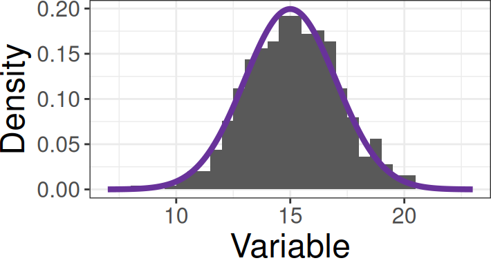
Hypothesis testing based on distributional assumptions

Table of Contents

• Links to the sections in this module:
  • General Procedures for Hypothesis Testing
  • Assumption of Normality & CLT
  • Testing One Proportion
  • Testing One Mean
  • Testing Two Proportions
  • Testing Two Independent Means
  • Testing Paired Means
  • Theory vs. Simulation Comparison

Learning objectives

By the end of this module, you will be able to:

• Conduct hypothesis tests for 1 and 2 samples (means & proportions) using normal and \(t\)-distributions.

• Compare theory-based (CLT) testing with simulation/resampling methods.

• Implement hypothesis tests in R using t.test(), prop.test(), and manual formulas.

• Evaluate the assumptions, validity conditions, and limitations of theory-based inference.

Review: inferential goals

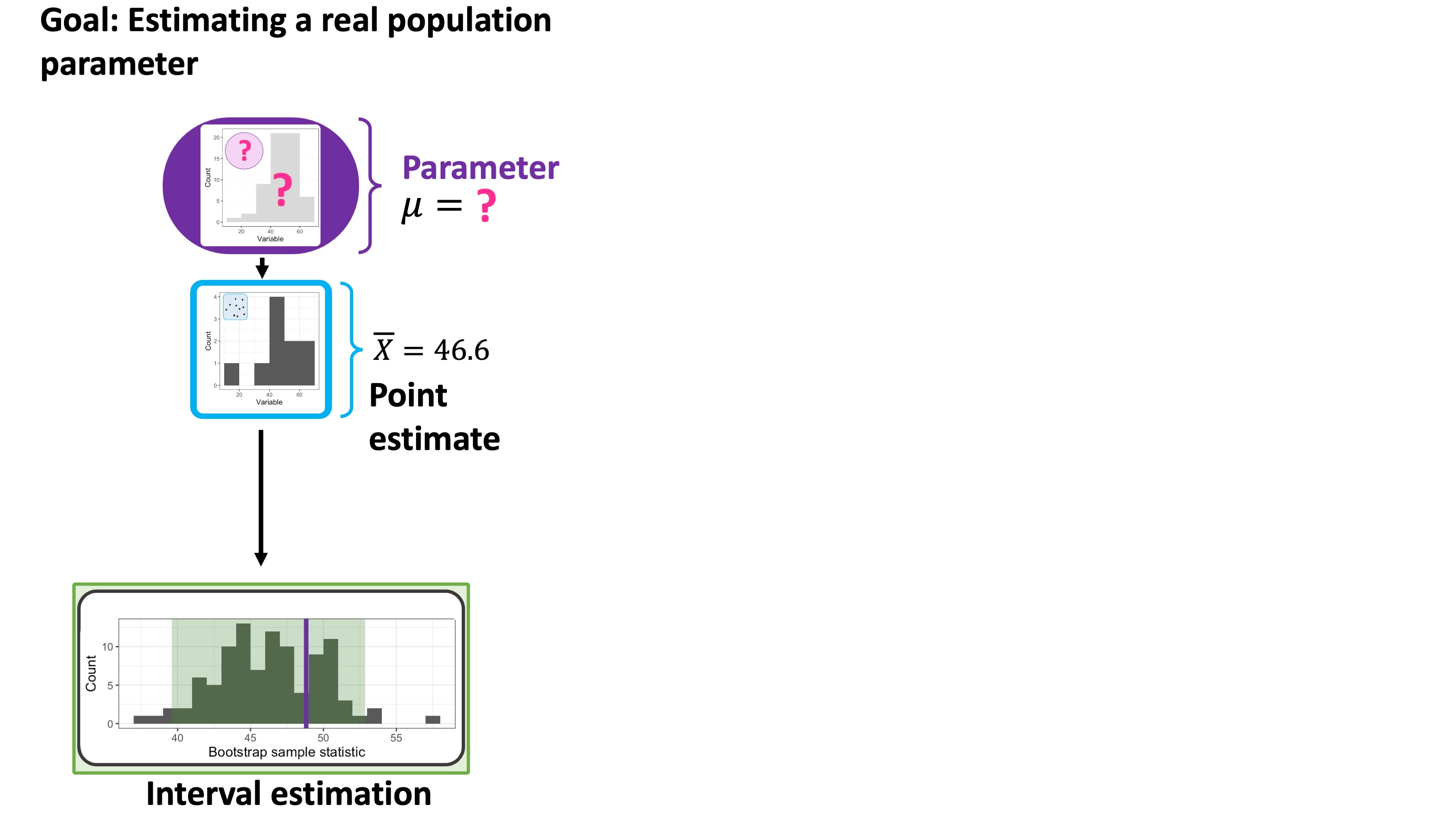
Review: inferential goals

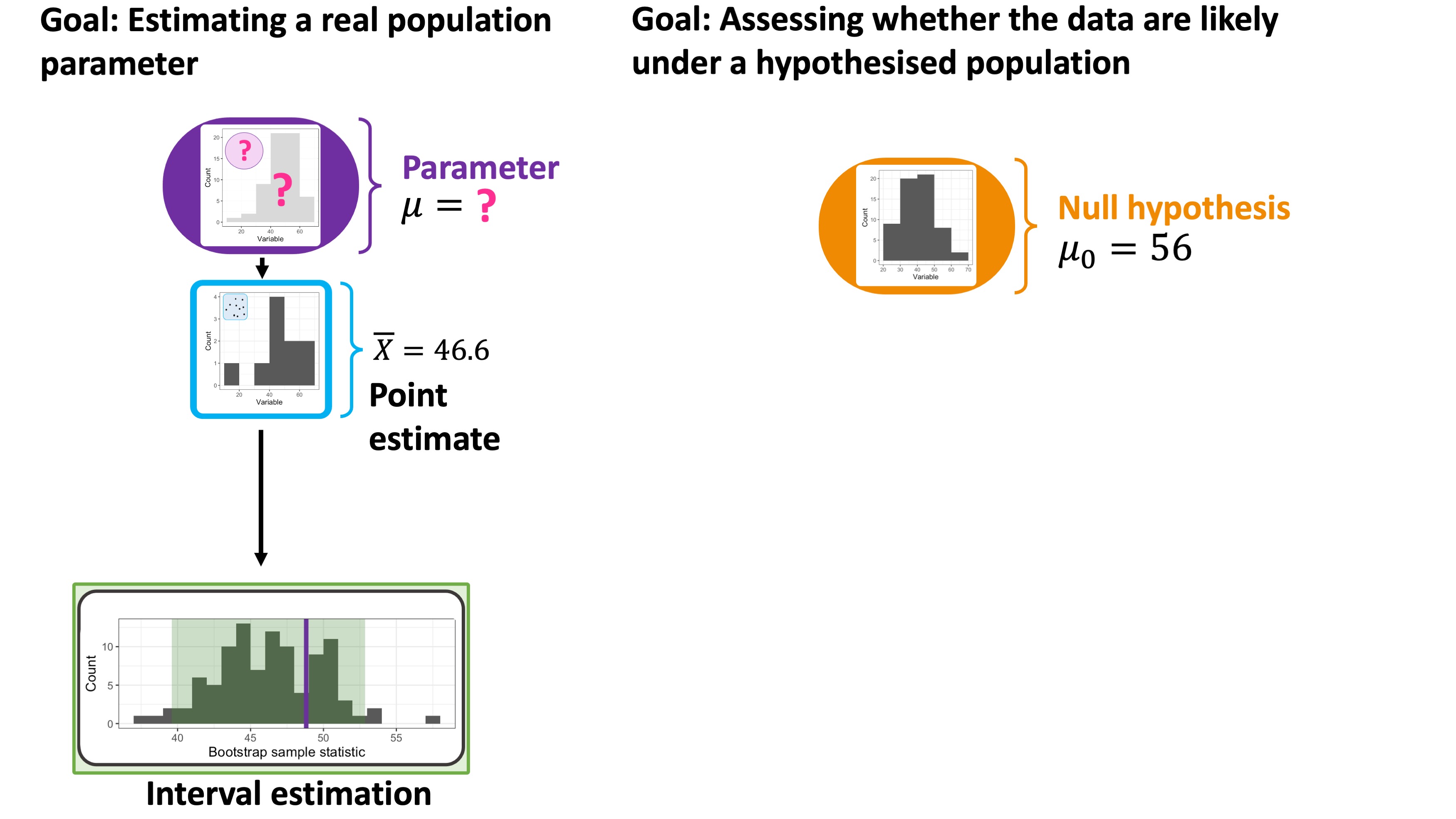
Review: inferential goals

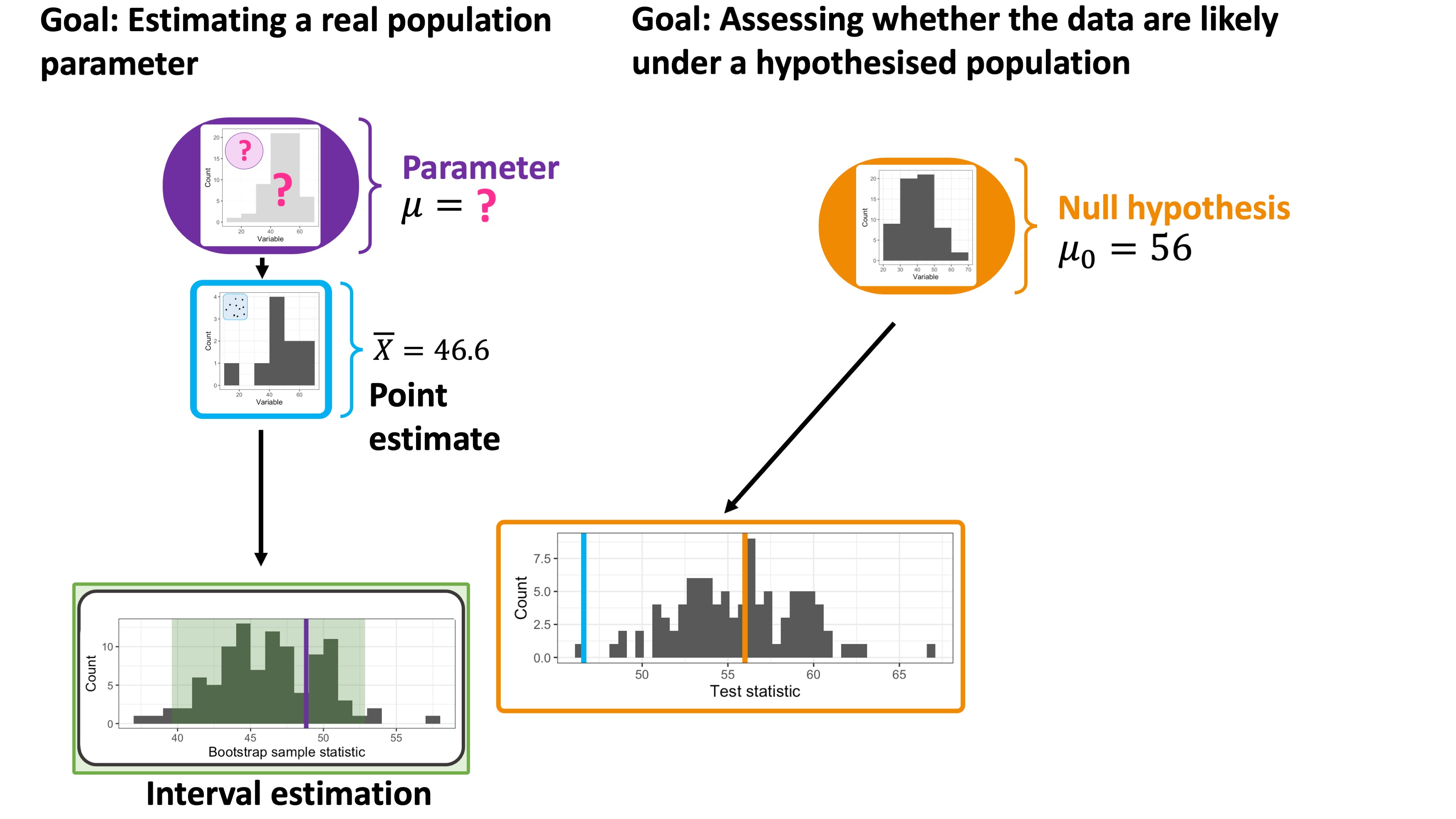
Review: inferential goals

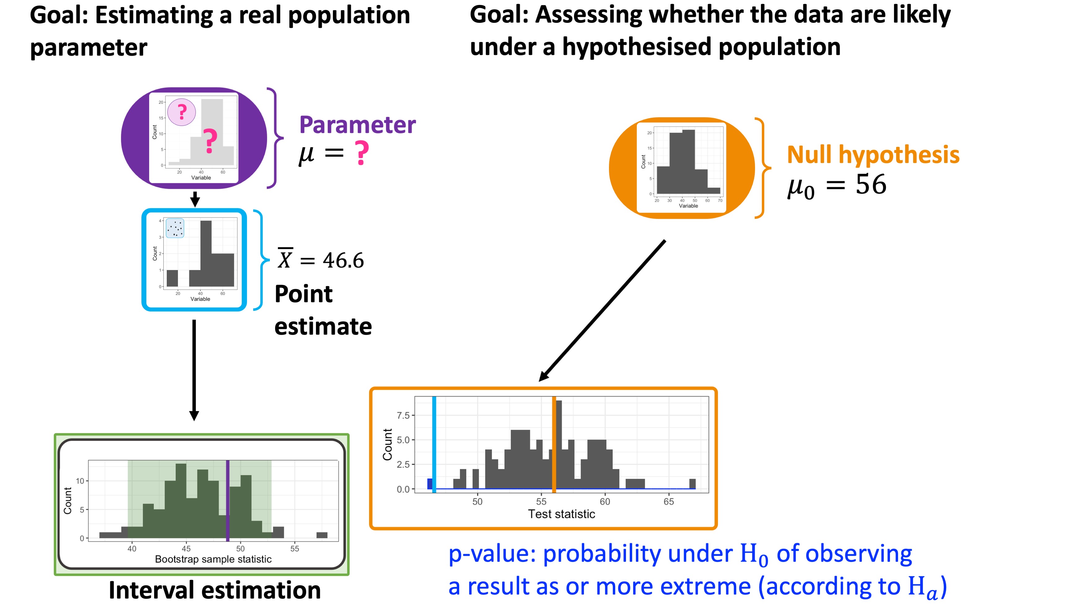
Review: inferential goals

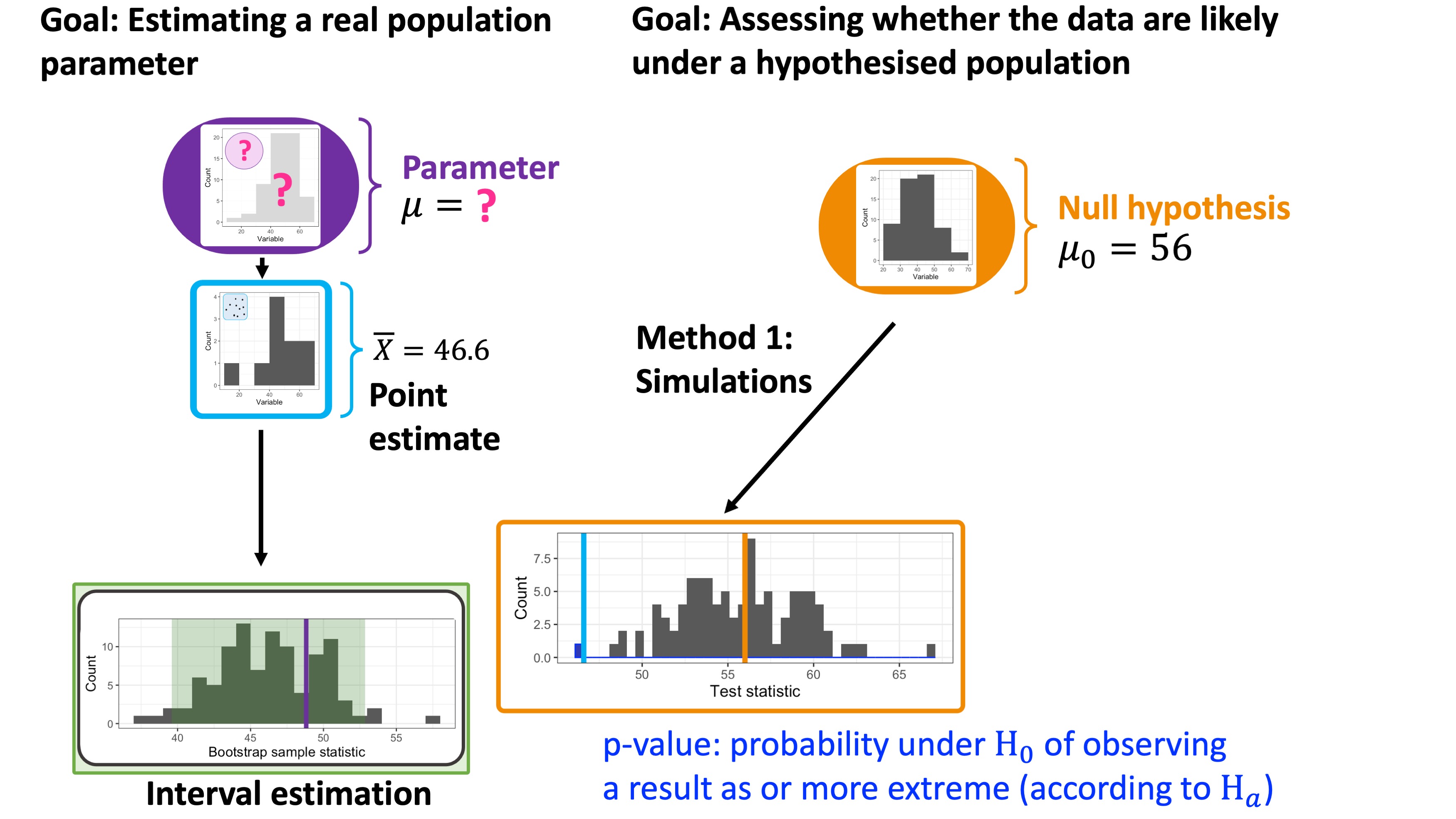
Review: inferential goals

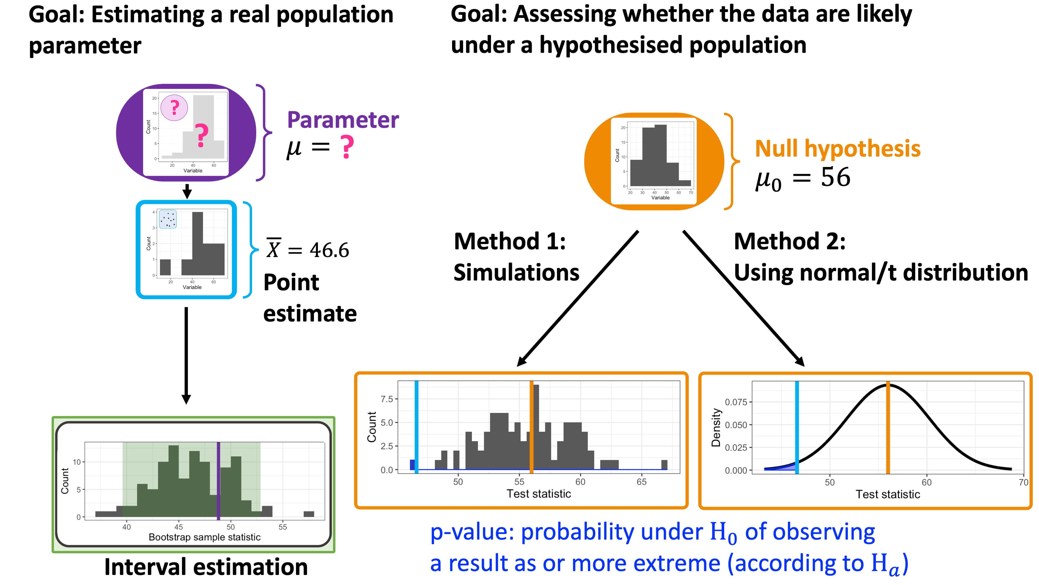
Today’s goal

• Our goal: use assumption of normality or the Central Limit Theorem to perform hypothesis testing

General procedures for null hypothesis testing

1. Define null and alternative hypotheses
2. Set significance level
3. Choose a test statistic
4. Find the null model
5. Calculate observed test statistic and associated \(p\)-value
6. Make a decision

General procedures for null hypothesis testing

1. Define null and alternative hypotheses

2. Set significance level

3. Choose a test statistic

4. Find the null model

5. Calculate observed test statistic and associated \(p\)-value

6. Make a decision

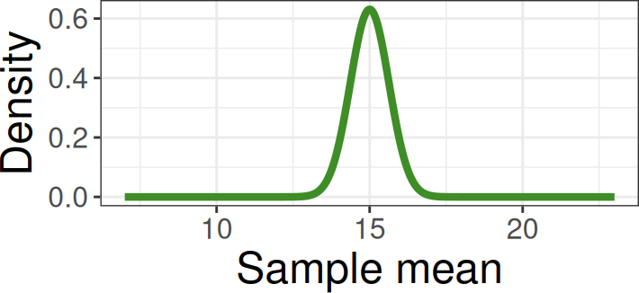
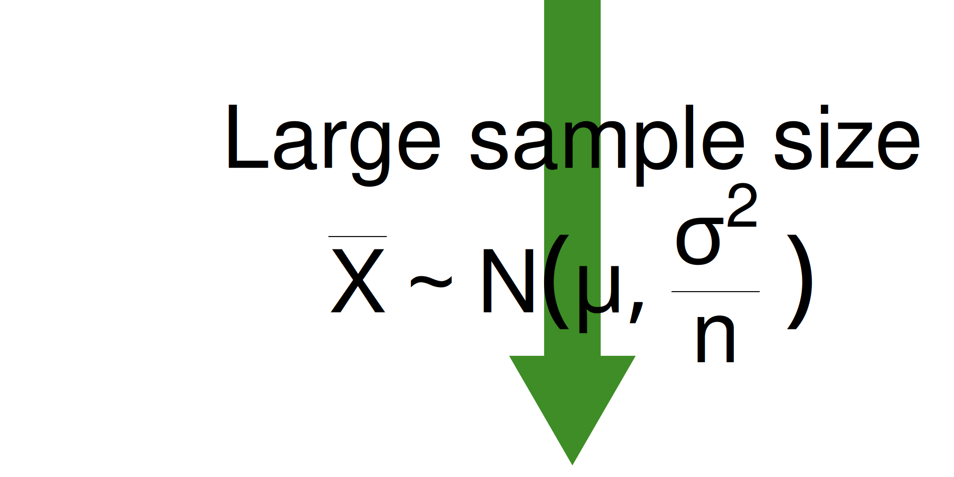
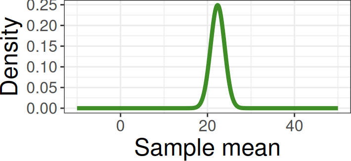
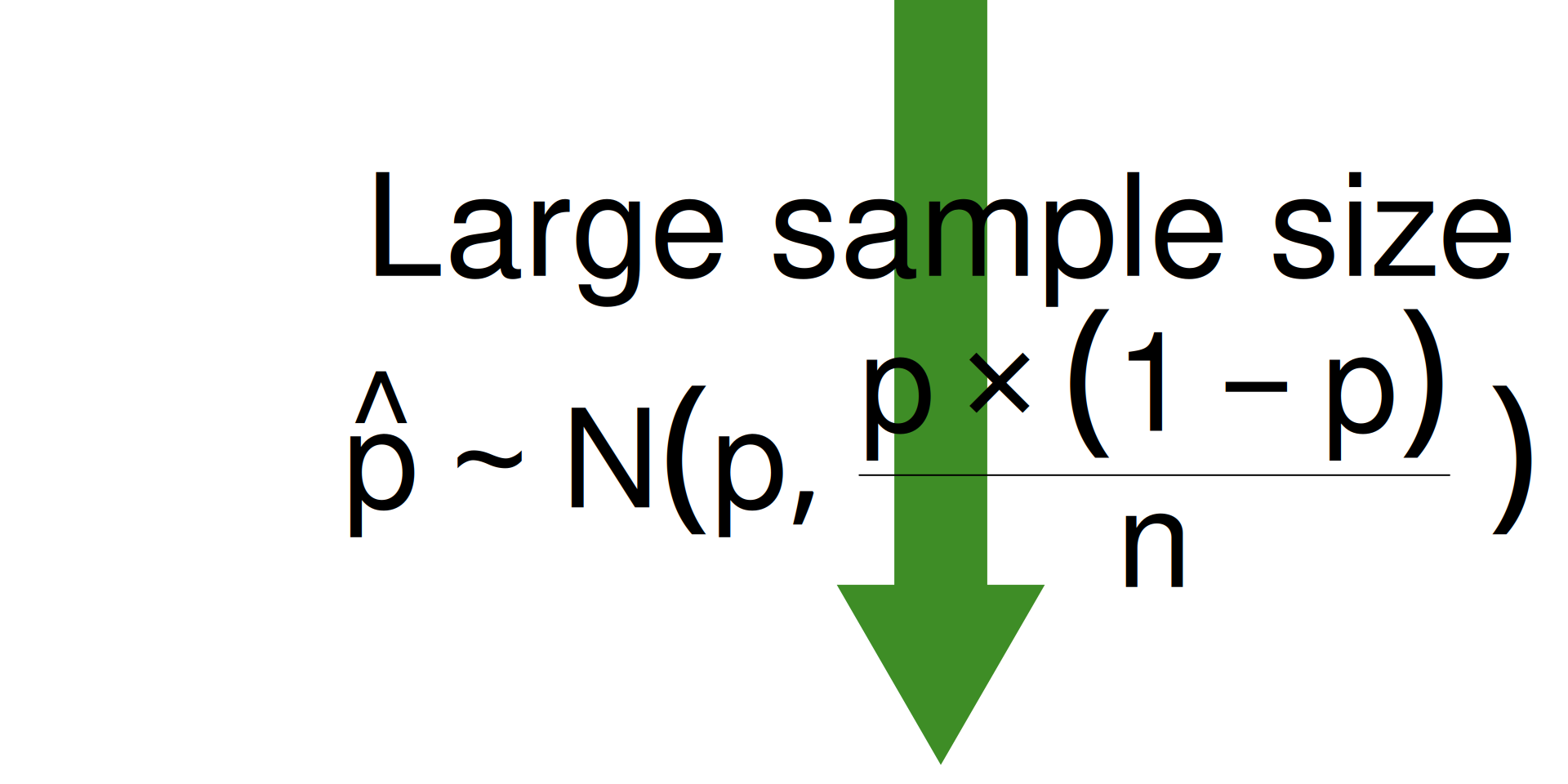
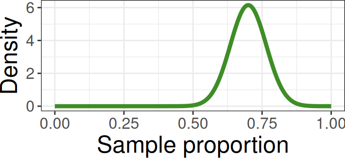
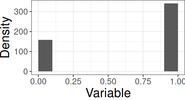
Assumption of normality and central limit theorem

Normal population

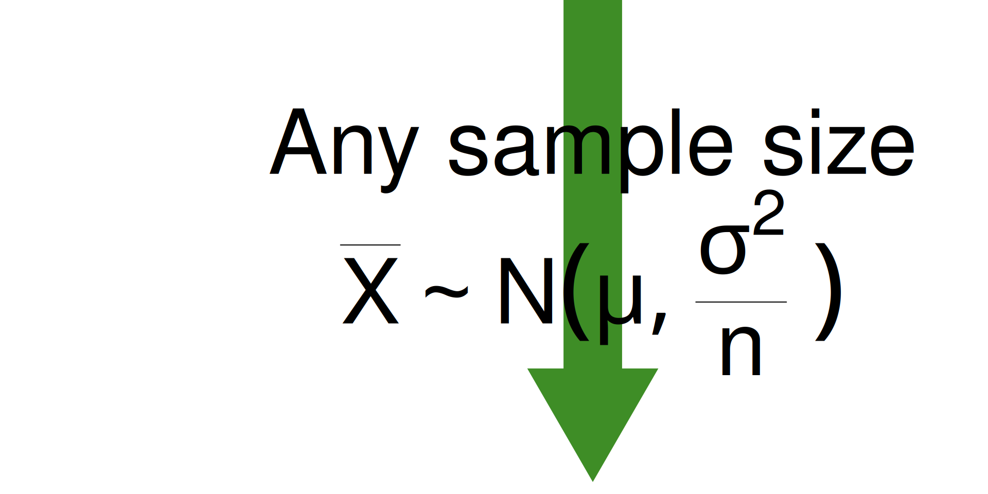
Any population

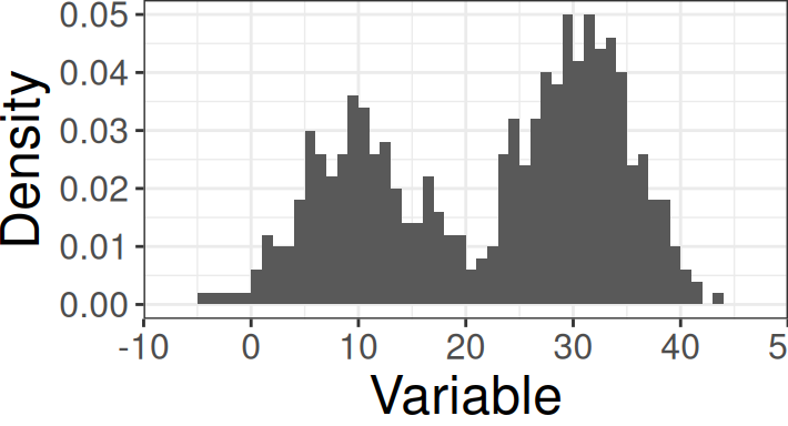
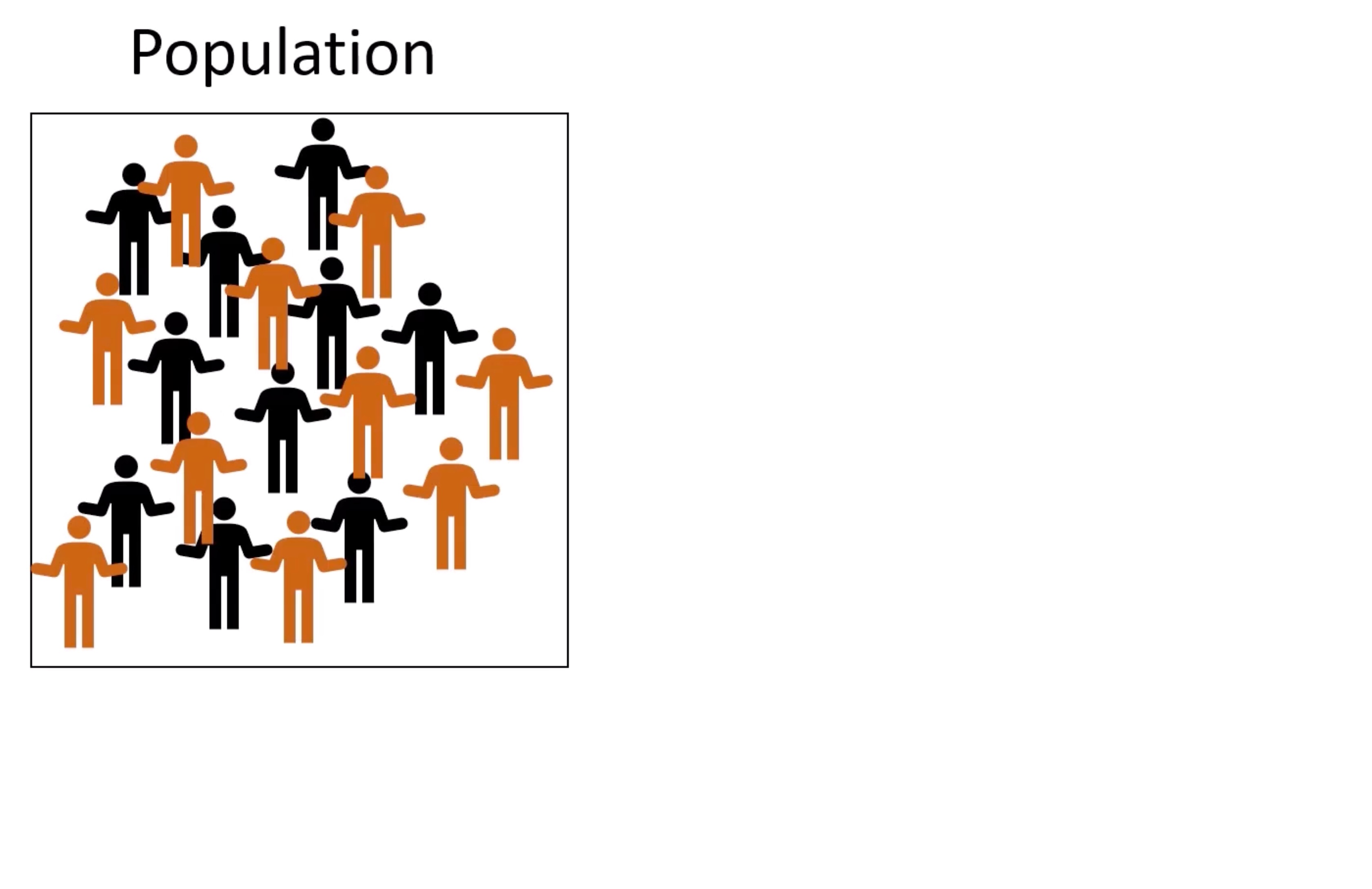
Population (binary)

Testing one proportion

Example: Coin Flip

Scroll down

Your friend claims that they have psychic abilities and can predict the outcome of coin flips before they happen. You decide to test them by flipping a coin 100 times, and count the number of times they guessed right.

Step 1: Define null and alternative hypotheses

• \(H_0: p = 0.5\) vs. \(H_A: p > 0.5\)

Step 2: Specify the significance level

• Let’s set the significance level at 10%

Step 3: Choose a test statistic

• Since we are testing a proportion, we can use \(\hat{p}\).

Step 4: Find the null model

• If we assume \(H_0\) to be true, we have that \(p = p_0\). In that case, based on the CLT:

\[\hat{p} \sim N \left(p_0, \frac{p_0 (1-p_0)}{n} \right)\]

• Check:
  • \(n\times p_0 \ge 10\) and \(n\times(1 − p_0) \ge 10\)
  • Here, \(100\times 0.5 = 50 \ge 10\) and \(100\times (1 - 0.5) = 50 \ge 10\) ✅
  • necessary conditions (random, independent)

• In this example, \(H_0: p = 0.5\), therefore \(p_0 = 0.5\), consequently under \(H_0\) we have:

\[\hat{p} \sim N \left(0.5, \frac{0.5\times0.5}{100} \right)\]

Step 5: Compute the p-value

• Your friend correctly predicts 55 out of 100 flips. How unusual is \(\hat{p} = 0.55\) under our null model?

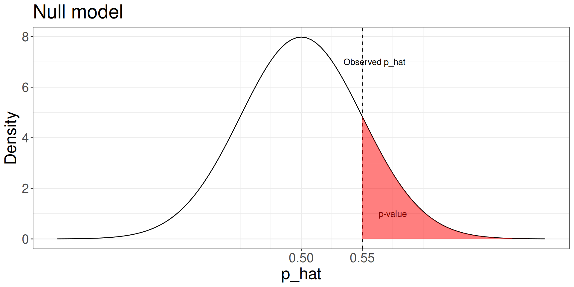
(p_value <- pnorm(0.55, 0.5, sqrt((0.5*0.5)/100), lower.tail = FALSE))

[1] 0.1586553

Step 6: Make a decision

• Since the \(p\)-value > 0.10, we do not reject \(H_0\) and conclude that:

There is not enough evidence, at \(10\%\) significance level, to suggest that your friend’s guesses were better than random guessing

Review: p-value

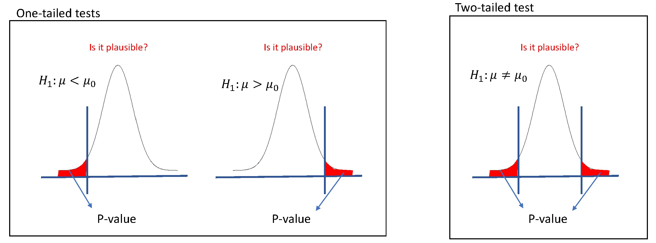
• \(p\)-value:
  • summarizes the evidence
  • describes how unusual the data would be if \(H_0\) were true
  • defined as the probability of observing a result as extreme or more extreme towards the alternative hypothesis than what we observed given that \(H_0\) is true

CLT and Standardization

• When relying on the CLT, we usually use a standardized version of the test statistic;

• For example, instead of using \(\hat{p} \sim N\left(p_0, \frac{p_0(1-p_0)}{n}\right)\), we use the z-score: \[Z = \frac{\hat{p} - p_0}{\sqrt{\frac{p_0(1-p_0)}{n}}}\sim N(0,1)\]

• The advantage of doing this is that we can use the same process for the proportion, mean, difference in proportion, and difference in means.

Example - Coin Flip - Revisited

Scroll down

Your friend claims that they have psychic abilities and can predict the outcome of coin flips before they happen. You decide to test them by flipping a coin 100 times, and count the number of times they guessed right.

Step 1: Define null and alternative hypotheses

• \(H_0: p = 0.5\) vs. \(H_A: p > 0.5\)

Step 2: Specify the significance level

• Let’s set the significance level at 10%

Step 3: Choose a test statistic

• Since we are testing a proportion, we will use

\[Z = \frac{\hat{p} - p_0}{\sqrt{\frac{p_0(1-p_0)}{n}}}\]

Step 4: Find the null model

• If we assume \(H_0\) to be true, we have that \(p = p_0\). In that case, based on the CLT:

\[Z \sim N \left(0, 1\right)\]

• Check:
  • \(n\times p_0 \ge 10\) and \(n\times(1 − p_0) \ge 10\)
  • necessary conditions (random, independent)

Step 5: Compute the p-value

• Your friend correctly predicts 55 out of 100 flips. How unusual is \(\hat{p} = 0.55\) under our null model? \[Z = \frac{0.55 - 0.5}{0.05} = 1\]

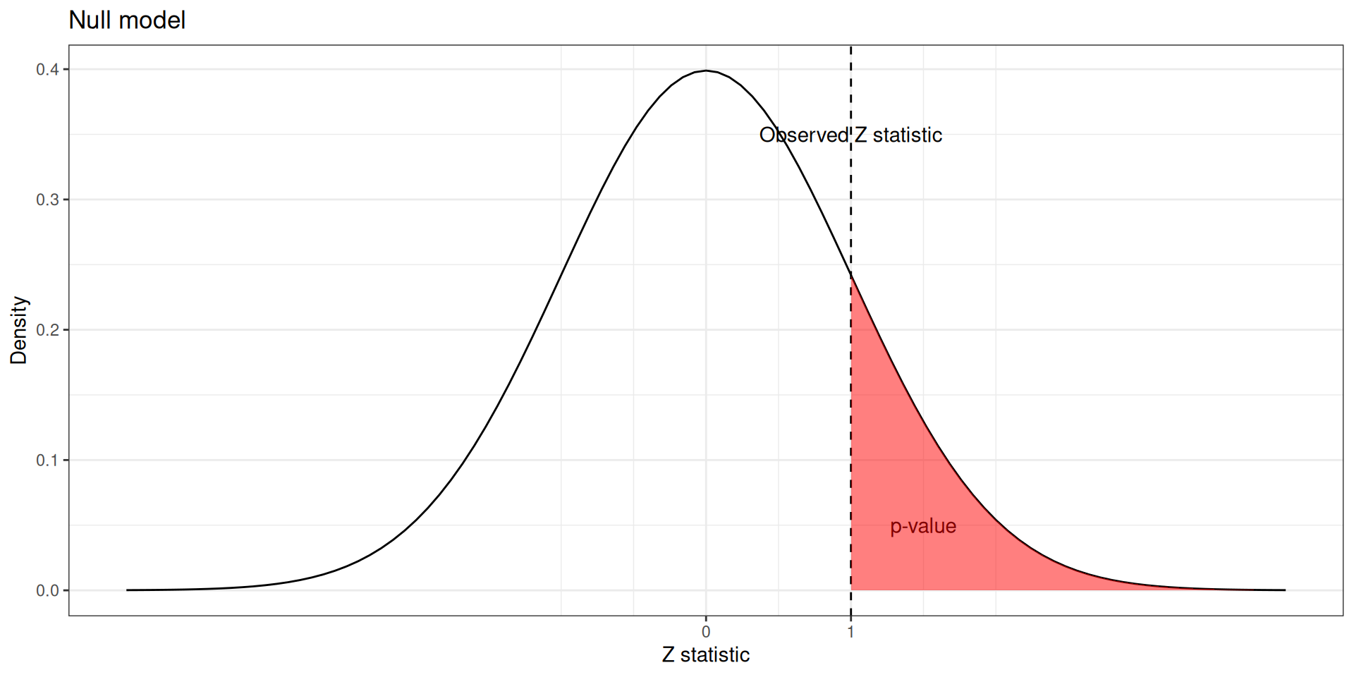
(p_value <- pnorm(1, lower.tail = FALSE))

[1] 0.1586553

• Note we got the exactly same p-value;
  • the tests are equivalent.

Step 6: Make a decision

• Since the \(p\)-value > 0.10, we do not reject \(H_0\) and conclude that:

There is not enough evidence, at \(10\%\) significance level, to suggest that your friend’s guesses were better than random guessing

R Code: Testing One Proportion

We can use prop.test() to perform the hypothesis test interactively:

• Reading the Output:
  • X-squared = 1: The \(Z\)-statistic is \(Z = \sqrt{\text{X-squared}} = \sqrt{1} = 1.0\).
  • p-value = 0.1587: Matches our manual calculation pnorm(1, lower.tail = FALSE).

Your Turn: Left-Handed Tennis Players

About \(10\%\) of the general population is left-handed, yet left-handers show up more often among elite fencers, boxers, and tennis players — a pattern some researchers attribute to the element of surprise a left-handed opponent brings against right-handed-dominated competition. A sports analyst samples \(n = 200\) players from a professional tennis ranking list and finds that \(28\) of them play left-handed. Is there evidence that left-handedness is over-represented among these professional players, compared to the general population rate of \(10\%\)?

\[H_0: p = 0.10 \quad \text{vs.} \quad H_A: p > 0.10, \qquad \alpha = 5\%\]

Part (a): Compute the test statistic and \(p\)-value by hand

Given: \(x = 28\) left-handed players out of \(n = 200\) sampled, testing against \(p_0 = 0.10\). Fill in the blanks below to walk through the computation.

The sample proportion is the number of successes divided by the sample size: \(\hat{p} = x/n\).

Under \(H_0\), the standard error uses the hypothesized proportion \(p_0\), not \(\hat{p}\): \(SE = \sqrt{p_0(1-p_0)/n}\).

The \(Z\) test statistic standardizes the distance between \(\hat{p}\) and \(p_0\): \(Z = (\hat{p} - p_0)/SE\).

Since \(H_A: p > p_0\), the \(p\)-value is the area to the right of your observed \(Z\) under the standard normal curve: pnorm(z, lower.tail = FALSE).

phat <- x / n
se <- sqrt(p0 * (1 - p0) / n)
z <- (phat - p0) / se
pval <- pnorm(z, lower.tail = FALSE)
list(phat = phat, se = se, z = z, pval = pval)

Your Turn: Left-Handed Tennis Players – R Code

Now confirm your hand calculation using prop.test().

prop.test() needs the number of successes (x), the sample size (n), and the hypothesized proportion (p).

Since \(H_A: p > 0.10\) is one-sided in the “greater” direction, set alternative = "greater".

Full call: prop.test(x = 28, n = 200, p = 0.10, alternative = "greater", correct = FALSE).

prop.test(x = 28, n = 200, p = 0.10, alternative = "greater", correct = FALSE)

Testing one mean

Example: Coffee Shop

Scroll down

Alice, the coffee shop owner, wants to see if her new marketing campaign increased her average daily latte sales, which were 50 before the campaign. After 25 days, the average sales increased to 55 lattes per day, with a sample standard deviation of 8.

Step 1: Define null and alternative hypotheses

• \(H_0: \mu = 50\) vs. \(H_A: \mu > 50\)

Step 2: Specify the significance level

• Let’s set the significance level at \(5\%\).

Step 3: Choose a test statistic

• We will use the \(t\)-statistic: \[T = \frac{\bar{X} - \mu_0}{S/\sqrt{n}}\]

Step 4: Find the null model

• If we assume \(H_0\) to be true, we have that \(\mu = \mu_0\). In that case, based on the CLT:

\[T \sim t_{n-1}\]

Assumptions and conditions:

• Sample is randomly drawn from the population.
• Sample values are independent.
  • If your sample size is greater than 10% of the population size, there will be a severe violation of independence.
• Normality:
  • When the underlying distribution of \(x\) is non-Normal or unknown, sample size must be large enough
  • When the underlying distribution of \(x\) is exactly or nearly Normal, using the t-model is justified with small sample sizes

Step 5: Compute the p-value

• Alice’s sample had \(\bar{X} = 55\) and \(S = 8\). The observed test statistic is:

\[T = \frac{55 - 50}{\frac{8}{\sqrt{25}}} = 3.125\]

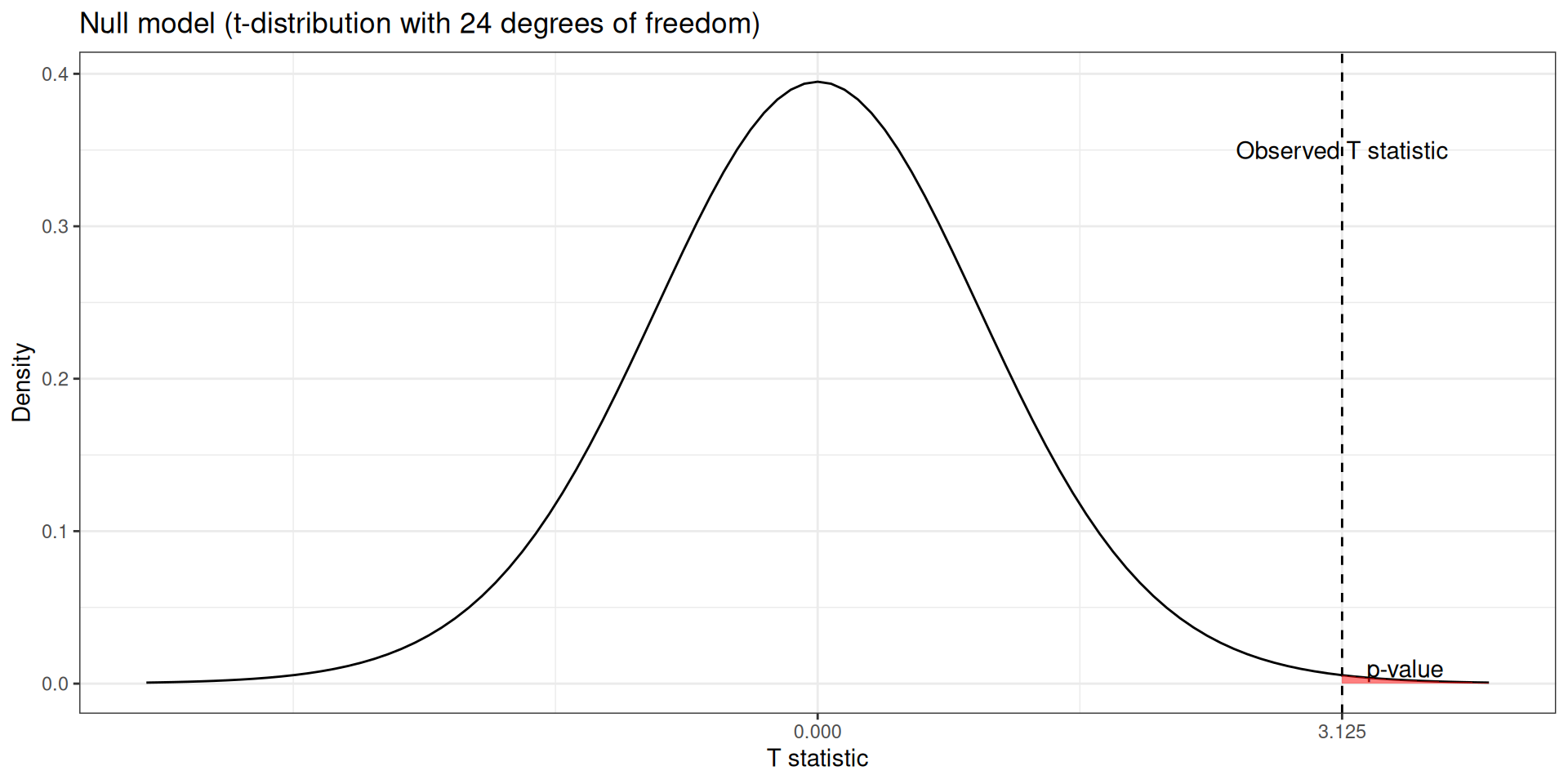
(p_value <- pt(3.125, 24, lower.tail = FALSE))

[1] 0.002301319

Step 6: Make a decision

• Since the \(p\)-value \(< 5\%\), we reject \(H_0\) and conclude that:

There is sufficient evidence, at \(5\%\) significance level, to conclude that the average daily latte sales have increased after the new marketing campaign.

R Code: Testing One Mean

The \(25\) daily sales figures are stored in the latte_data data frame (column sales).

• Extracting Quantities:
  • res_latte$statistic: The calculated \(T\)-statistic (\(T = 3.125\)).
  • res_latte$parameter: Degrees of freedom (\(df = n - 1 = 24\)).
  • res_latte$p.value: \(p\)-value for testing if daily sales increased.

Your Turn: Wireless Earbud Battery Life

A manufacturer advertises that its new wireless earbuds last, on average, \(8\) hours per charge under continuous use. A tech reviewer is skeptical of the claim and tests a sample of \(n = 20\) units, measuring how long each lasts before dying. The sample mean is \(\bar{x} = 7.5\) hours with a sample standard deviation of \(s = 1.1\) hours. Is there evidence that the manufacturer is overstating the battery life?

\[H_0: \mu = 8 \quad \text{vs.} \quad H_A: \mu < 8, \qquad \alpha = 5\%\]

Part (a): Compute the test statistic and \(p\)-value by hand

Given: \(n = 20\), \(\bar{x} = 7.5\), \(s = 1.1\), testing against \(\mu_0 = 8\).

For a one-sample \(t\)-test, the degrees of freedom are \(n - 1\).

The standard error of the sample mean is \(s / \sqrt{n}\).

The \(T\) statistic is \(T = (\bar{x} - \mu_0) / SE\).

Since \(H_A: \mu < \mu_0\), the \(p\)-value is the area to the left of your observed \(T\) under a \(t_{df}\) distribution: pt(t_stat, df) (the default is the lower tail).

df <- n - 1
t_stat <- (xbar - mu0) / (s / sqrt(n))
pval <- pt(t_stat, df)
list(df = df, t_stat = t_stat, pval = pval)

Your Turn: Wireless Earbud Battery Life – R Code

The reviewer’s \(20\) battery-life measurements are stored in the battery_life vector.

t.test() needs the sample vector and the hypothesized mean (mu).

Since \(H_A: \mu < 8\), set alternative = "less".

Full call: t.test(battery_life, mu = 8, alternative = "less").

t.test(battery_life, mu = 8, alternative = "less")

Testing two proportions

Example: Cigarette

Scroll down

Example from: https://online.stat.psu.edu/stat415/lesson/9/9.4 (Pennsylvania State University)

Via a telephone poll, Time magazine asked 800 adult Americans:

“Should the federal tax on cigarettes be raised to pay for health care reform?”

The results of the survey were:

• 351 out of 605 non-smokers said “yes”
• 41 out of 195 smokers said “yes”

Is there sufficient evidence at the \(\alpha = 0.05\) to conclude that the two populations differ significantly with respect to their opinions?

Step 1: Define null and alternative hypotheses

The hypotheses are: \[H_0: p_1 - p_2 = 0\quad \text{vs.} \quad H_A: p_1 - p_2 \neq 0\]

• \(p_1\): proportion of the non-smoker population who reply “yes”

• \(p_2\): proportion of the smoker population who reply “yes”

Step 2: Specify the significance level

• The significance level was specified as \(\alpha = 0.05\).

Step 3: Choose a test statistic

• The test statistic we will use is: \[Z = \frac{\hat{p}_1 - \hat{p}_2}{\sqrt{\hat{p} \left(1 -\hat{p}\right)\left( \frac{1}{n_1} + \frac{1}{n_2}\right)}}\]

where \(\hat{p}\) is the overall sample proportion, i.e., \(\hat{p} = \frac{\# Successes}{\# Total}\) (considering both groups).

Step 4: Find the null model

• If we assume \(H_0\) to be true, for large samples we have that:

\[Z \sim N \left(0, 1\right)\]

Step 5: Compute the p-value

Observed proportions:

• Non-smokers: \(\hat{p}_1 = \frac{351}{605} = 0.58\)

• Smokers: \(\hat{p}_2 = \frac{41}{195} = 0.21\)

• Overall sample proportion: \(\hat{p} = \frac{351 + 41}{605 + 195} = 0.49\)

Observed test statistic:

\[ Z = \frac{0.58 - 0.21}{\sqrt{0.49\times 0.51\left( \frac{1}{605} + \frac{1}{195}\right)}} = 8.99\]

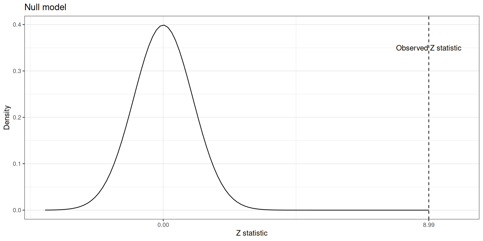
observed_test_statistic <- 8.99

(p_value <- 2*pnorm(abs(observed_test_statistic), lower.tail = FALSE))

[1] 2.472304e-19

Step 6: Make a decision

• Since the \(p\)-value \(\leq 0.05\), we reject \(H_0\) and conclude that:

There is sufficient evidence at the \(5\%\) significance level to conclude that the two populations differ with respect to their opinions concerning imposing a federal tax to help pay for health care reform.

R Code: Testing Two Proportions

For two independent proportions (Non-smokers: 351/605 vs Smokers: 41/195):

• Connecting Math to R Output:
  • X-squared = 80.82: Taking \(\sqrt{80.82} = 8.99\), which is our \(Z\)-statistic!
  • res_2prop$estimate: \(\hat{p}_1 = 0.580\) (non-smokers) and \(\hat{p}_2 = 0.210\) (smokers).

Your Turn: Email Subject Line A/B Test

A nonprofit is A/B testing two subject lines for its fall fundraising email. Subject line A is sent to \(500\) recipients and opened by \(40\) of them. Subject line B is sent to a different \(500\) recipients and opened by \(65\). Is there evidence that the two subject lines have different open rates?

\[H_0: p_1 - p_2 = 0 \quad \text{vs.} \quad H_A: p_1 - p_2 \neq 0, \qquad \alpha = 5\%\]

• \(p_1\): true open rate for subject line A
• \(p_2\): true open rate for subject line B

Part (a): Compute the test statistic and \(p\)-value by hand

\(\hat{p}_1 = x_1/n_1\) and \(\hat{p}_2 = x_2/n_2\).

The pooled proportion combines the successes from both samples: \(\hat{p} = (x_1 + x_2)/(n_1 + n_2)\).

\(SE = \sqrt{\hat{p}(1-\hat{p})\left(\frac{1}{n_1} + \frac{1}{n_2}\right)}\), using the pooled proportion, not \(\hat{p}_1\) or \(\hat{p}_2\) individually.

\(Z = (\hat{p}_1 - \hat{p}_2)/SE\).

Since \(H_A\) is two-sided (\(\neq\)), the p-value is twice the upper-tail area: 2 * pnorm(abs(z), lower.tail = FALSE).

p1_hat <- x1 / n1
p2_hat <- x2 / n2
p_pool <- (x1 + x2) / (n1 + n2)
se <- sqrt(p_pool * (1 - p_pool) * (1/n1 + 1/n2))
z <- (p1_hat - p2_hat) / se
pval <- 2 * pnorm(abs(z), lower.tail = FALSE)
list(p1_hat = p1_hat, p2_hat = p2_hat, p_pool = p_pool, se = se, z = z, pval = pval)

Your Turn: Email Subject Line A/B Test – R Code

Confirm your hand calculation using prop.test().

Pass both counts as a vector to x and both sample sizes as a vector to n, in the same order: x = c(x1, x2), n = c(n1, n2).

Since \(H_A\) is two-sided, set alternative = "two.sided".

Full call: prop.test(x = c(40, 65), n = c(500, 500), alternative = "two.sided", correct = FALSE).

prop.test(x = c(40, 65), n = c(500, 500), alternative = "two.sided", correct = FALSE)

Testing two means

Comparing mean of two groups

• To discuss the difference in means, we need to consider the relationship between the two groups.

• If the two groups are independent, we use the Welch’s two-sample t-test.

• If the two groups are dependent, we use the paired t-test.

Independent groups

• We want to see if people tend to marry later in life in the US compared to Canada.

• We want to compare the red cells count in healthy people and people with leukemia.

• We want to compare how much money Apple users are willing to spend on a new phone compared to Samsung users.

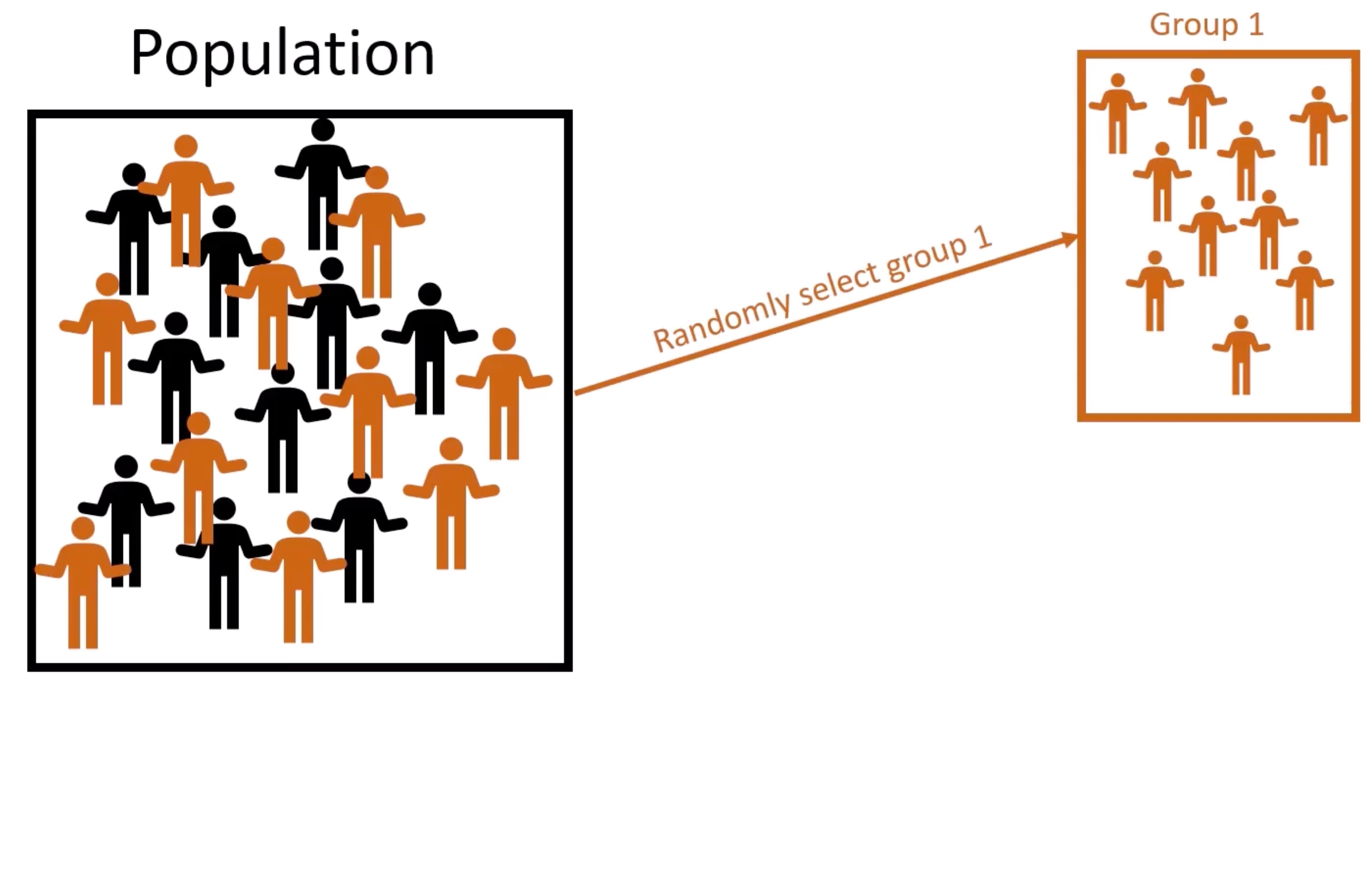
• In all these cases, one group has nothing to do with the other group.

Independent groups

Independent groups

Independent groups

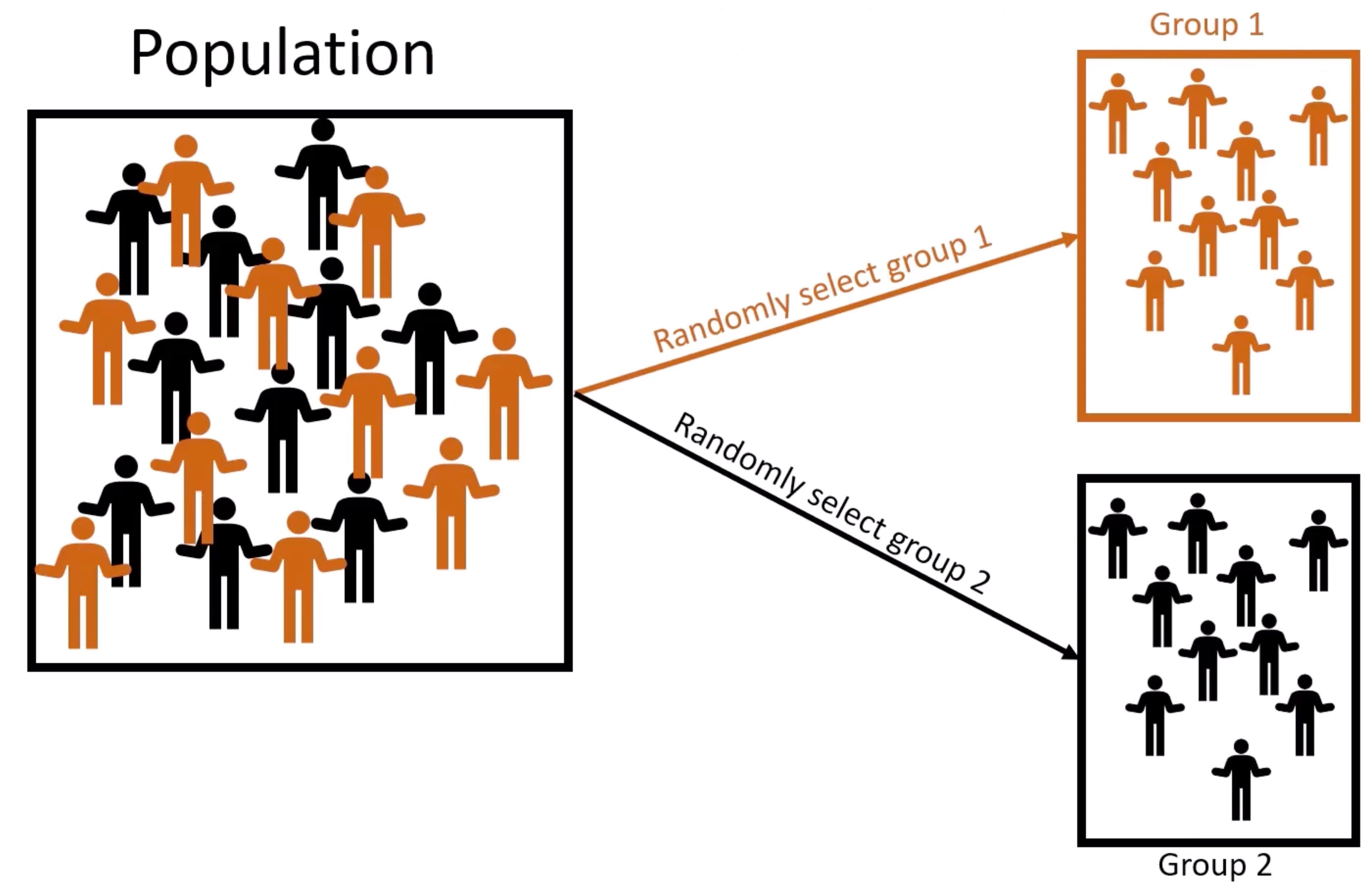
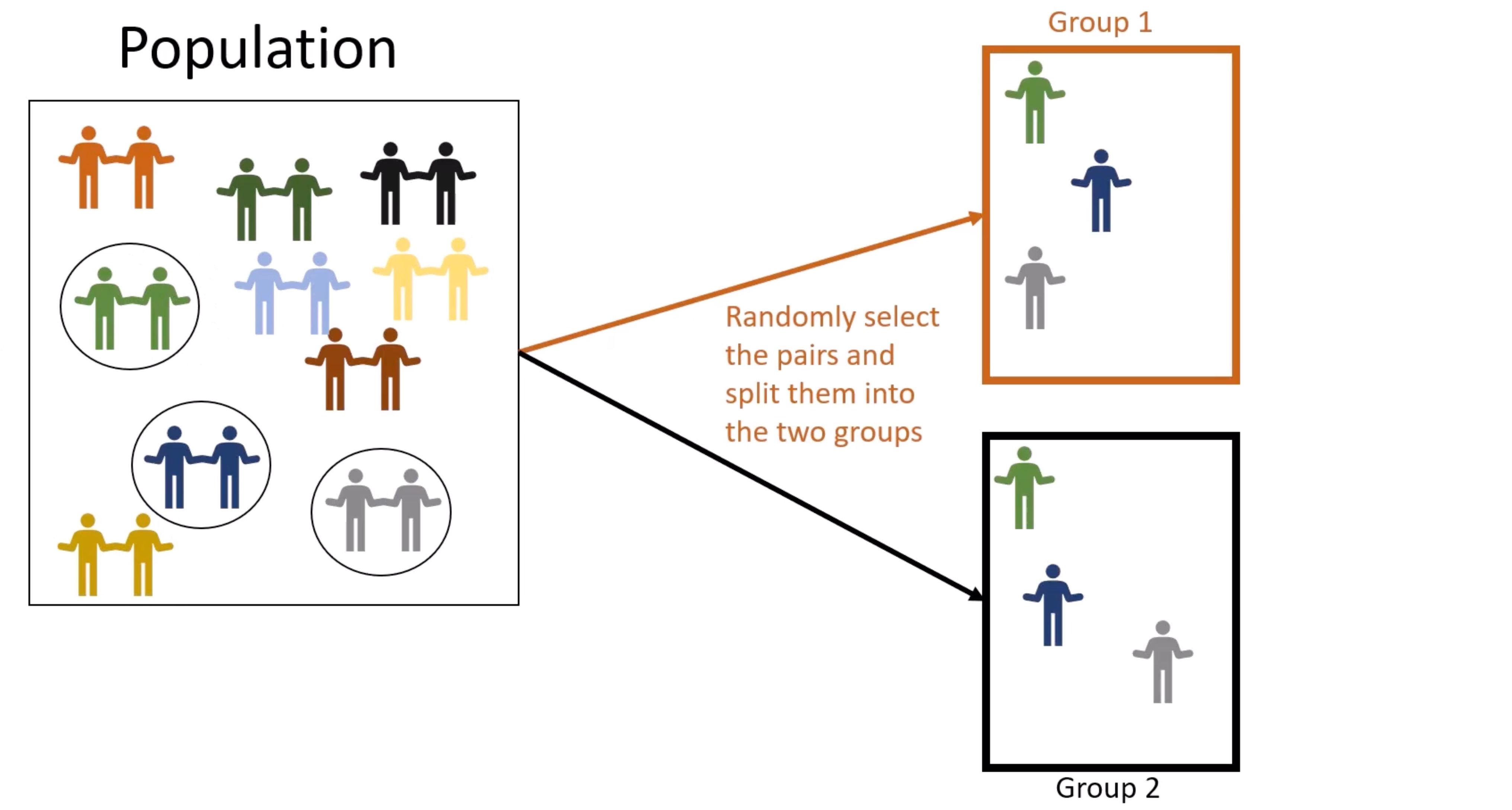
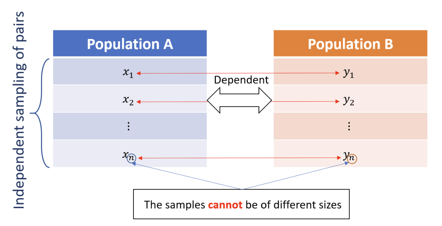
Dependent groups

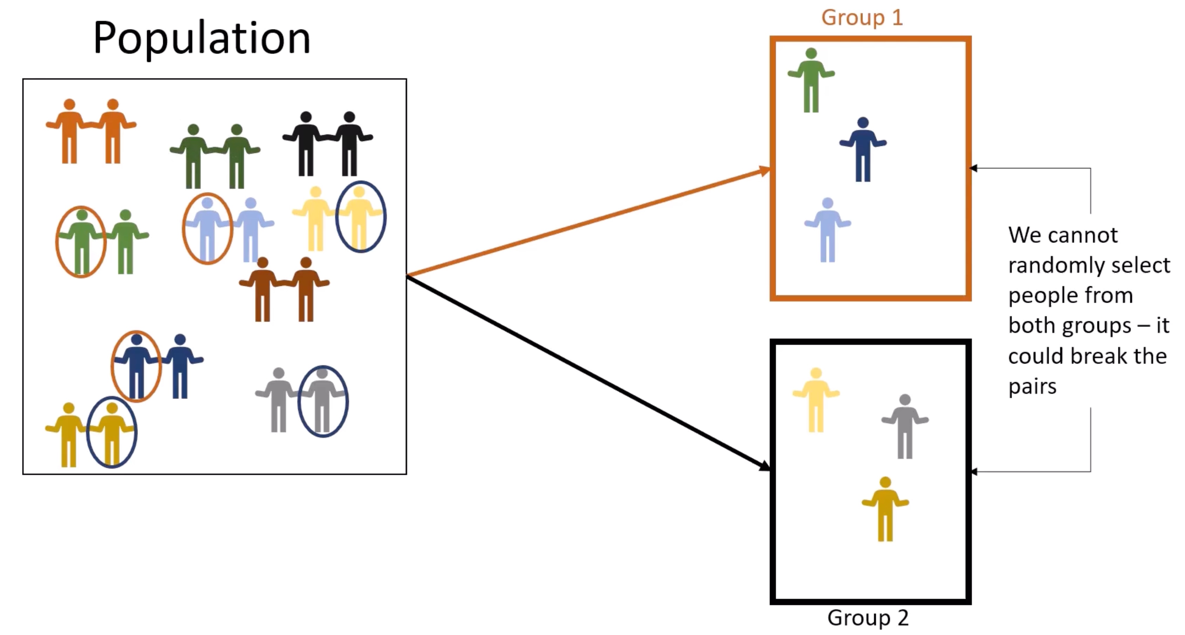
• We want to see if a new drug is effective in reducing blood pressure. We measure the blood pressure before the treatment and after the treatment.

• We want to see if married people have similar IQ levels.

• We want to compare the weight of twins at birth.

• In all these cases, the elements in one group are related to the elements in the other group.

Dependent groups

Dependent groups

Testing two independent means

Example: Independent Groups

Scroll down

• A researcher wants to investigate whether there’s a difference in the average daily screen time between teenagers in urban and rural areas.

• The researcher randomly samples 20 teenagers from urban areas and 25 teenagers from rural areas. They ask each teenager to report their average daily screen time (in hours) over the past week.

• The results of the survey were:

Group	Sample size	Sample mean	Std Dev
Urban	20	6.2 hours	1.5 hours
Rural	25	5.5 hours	1.2 hours

• Is there sufficient evidence at the \(\alpha = 10\%\) to conclude that the average daily screen time differs between teenagers in urban and rural areas?

Step 1: Define null and alternative hypotheses

The hypotheses are: \[H_0: \mu_1 - \mu_2 = 0\quad \text{vs.} \quad H_A: \mu_1 - \mu_2 \neq 0\]

• \(\mu_1\): average screen time for teenagers in urban areas

• \(\mu_2\): average screen time for teenagers in rural areas

Step 2: Specify the significance level

• The significance level was specified as \(\alpha = 10\%\).

Step 3: Choose a test statistic

• The test statistic we will use is: \[T = \frac{\left(\bar{X}_1 - \bar{X}_2\right) - \Delta_0}{\sqrt{\frac{S_1^2}{n_1} + \frac{S_2^2}{n_2}}}\]

Step 4: Find the null model

• If we assume \(H_0\) to be true, then \(\mu_1-\mu_2 = \Delta_0\), for large samples we have that:

\[T \sim t_k\] where k is \[k = \frac{ \left(\color{red}{\frac{S^2_1}{n_1}} + \color{blue}{\frac{S^2_2}{n_2}}\right)^2 }{ \color{red}{\frac{S_1^4}{n_1^2(n_1-1)}} + \color{blue}{\frac{S_2^4}{n_2^2(n_2-1)}} } \]

Assumptions and conditions for validity of using the t-model:

1. The two samples are randomly drawn from their respective populations.
2. Sampled individuals within the same sample are independent of each other. Just check that two sample sizes are no greater than 10% of their respective population sizes.
3. Sample size:

• If both \(x_1\) and \(x_2\) follow the Normal model, there is no restriction on the sample sizes \(n_1\) and \(n_2\).

• If \(x_1\) and \(x_2\) are non-Normal or follow an unknown distribution, we need reasonably large sample sizes to validate the Normal approximation by the CLT as well as the use of the t-model.

4. The two samples must be independent of each other.

Step 5: Compute the p-value

Observed test statistic:

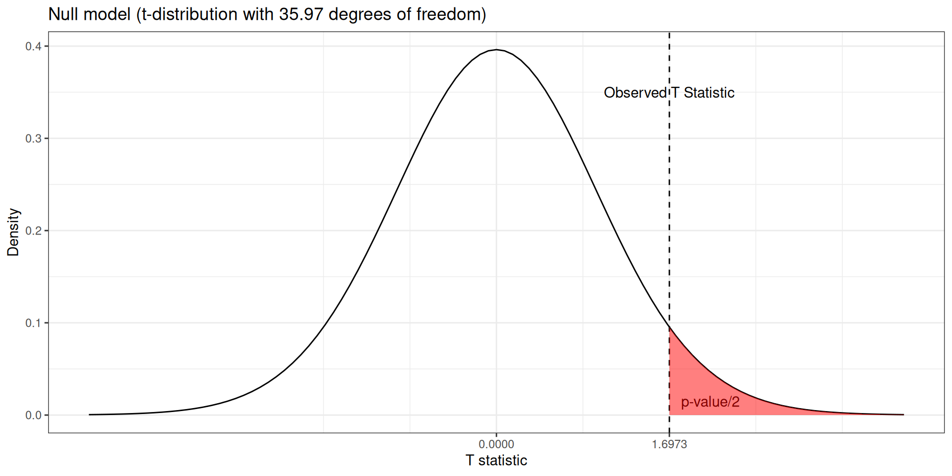
\[T = \frac{\left(6.2 - 5.5\right) - 0}{\sqrt{\frac{1.5^2}{20} + \frac{1.2^2}{25}}} \approx 1.6973\]

Degrees of freedom (\(k\)): \[k = 35.97\]

observed_test_statistic <- 1.6973

(p_value <- 2 * pt(abs(observed_test_statistic), 35.97, lower.tail = FALSE))

[1] 0.09827767

Step 6: Make a decision

• Since the \(p\)-value \(\leq 10\%\), we reject \(H_0\) and conclude that:

There is sufficient evidence to conclude that teenagers in urban and rural areas have different average daily screen times.

R Code: Testing Two Independent Means

The survey data is stored in the screen_data data frame (columns screen_time and area).

• Reading R’s t.test() Output:
  • screen_time ~ area: Formula syntax (response ~ group).
  • res_screen$parameter: Welch’s degrees of freedom (\(df \approx 35.97\)).

Your Turn: Study Hours, Online vs. In-Person

An instructor teaches two sections of the same course, one fully online and one in-person, and wants to know whether students in the two formats spend a different amount of time studying each week. A survey of \(n_1 = 18\) online students finds a mean of \(\bar{x}_1 = 6.8\) hours with \(s_1 = 2.1\) hours; a survey of \(n_2 = 22\) in-person students finds a mean of \(\bar{x}_2 = 5.9\) hours with \(s_2 = 1.6\) hours.

\[H_0: \mu_1 - \mu_2 = 0 \quad \text{vs.} \quad H_A: \mu_1 - \mu_2 \neq 0, \qquad \alpha = 5\%\]

• \(\mu_1\): average weekly study hours, online section
• \(\mu_2\): average weekly study hours, in-person section

Part (a): Compute the test statistic and \(p\)-value by hand

The Welch-Satterthwaite degrees of freedom formula is tedious to compute by hand, so it’s provided for you below in df.

\(SE = \sqrt{s_1^2/n_1 + s_2^2/n_2}\).

\(T = (\bar{x}_1 - \bar{x}_2)/SE\).

Since \(H_A\) is two-sided, the p-value is twice the upper-tail area under a \(t_{df}\) distribution: 2 * pt(abs(t_stat), df, lower.tail = FALSE).

se <- sqrt(s1^2/n1 + s2^2/n2)
t_stat <- (xbar1 - xbar2) / se
pval <- 2 * pt(abs(t_stat), df, lower.tail = FALSE)
list(se = se, t_stat = t_stat, pval = pval)

Your Turn: Study Hours, Online vs. In-Person – R Code

The survey data is stored in the study_data data frame (columns hours and format).

Use formula syntax response ~ group, i.e. hours ~ format.

Since \(H_A\) is two-sided, set alternative = "two.sided".

Full call: t.test(hours ~ format, data = study_data, alternative = "two.sided").

t.test(hours ~ format, data = study_data, alternative = "two.sided")

Testing paired means

Paired data

• The trick is to take the difference between the two groups and we can do a one-mean test for the differences.

Example: Paired Groups

Scroll down

• A fitness instructor wants to evaluate the effectiveness of a new 8-week training program designed to improve participants’ resting heart rate (RHR). They believe the program will lower RHR.

• The instructor recruits 12 participants and measures their RHR (in beats per minute) before starting the program and again after completing the 8-week program.

• The data is collected as follows:

Statistic	Before	After	Difference
Mean	73.42	72.62	0.8
Std Dev	5.16	5.23	1.07
n	12	12	12

Step 1: Define null and alternative hypotheses

The hypotheses are: \[H_0: \mu_1 - \mu_2 = 0\quad \text{vs.} \quad H_A: \mu_1 - \mu_2 > 0\]

• \(\mu_1\): average RHR before the program

• \(\mu_2\): average RHR after the program

Step 2: Specify the significance level

• Let’s set the significance level at \(\alpha = 1\%\).

Step 3: Choose a test statistic

• The test statistic we will use is: \[T = \frac{\bar{d} - \Delta_0}{\frac{s_d}{\sqrt{n}}}\]

• where:

  • \(\bar{d}\): mean of the within pair differences
  • \(s_d\): standard deviation of the within pair differences
  • \(n\): number of pairs

Step 4: Find the null model

• If we assume \(H_0\) to be true, then \(\mu_1-\mu_2 = \Delta_0\), for large samples we have that:

\[T \sim t_{n-1}\]

Assumptions and conditions for validity of using the t-model:

1. The n pairs are randomly drawn from the population.
2. The n pairs are independent of each other, i.e. any two distinct pairs are independent of each other. Just check that the number of pairs \(n\) is no greater than 10% of the population size.
3. Sample size

• If the within-pair differences (\(d_i\)) follow a Normal or nearly Normal distribution model, you can use the model even if the sample size \(n\) is small.
• If \(d_i\)’s follow an unknown or a non-Normal distribution, we need a reasonably large sample size \(n\) to validate the Normal approximation of \(\bar{d}\) by the CLT as well as the use of the t-model.

Step 5: Compute the p-value

Observed test statistic:

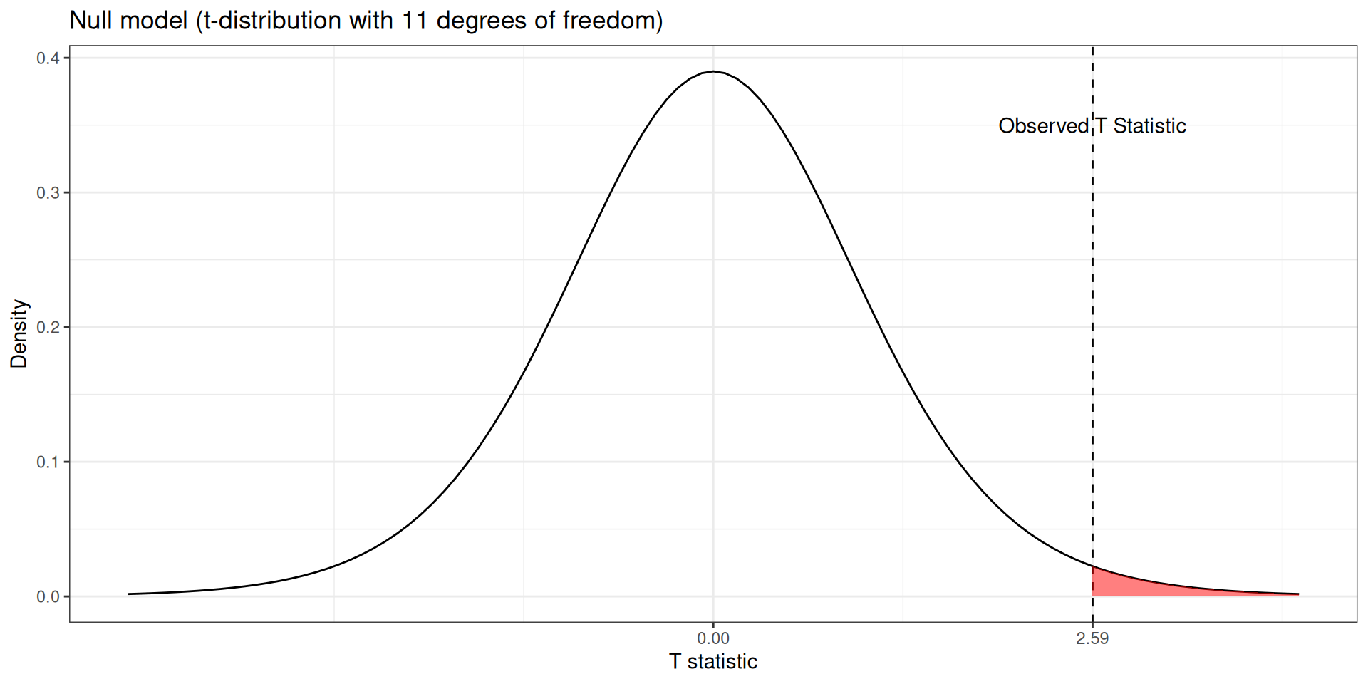
\[T = \frac{0.8 - 0}{\frac{1.07}{\sqrt{12}}} \approx 2.59\]

observed_test_statistic <- 2.59

(p_value <- pt(observed_test_statistic, 11, lower.tail = FALSE))

[1] 0.01256911

Step 6: Make a decision

• Since the \(p\)-value \(> 1\%\), we fail to reject \(H_0\) and conclude that:

There is not enough evidence, at \(\alpha = 1\%\), to conclude that the 8-week training program decreases participants’ average resting heart rate.

R Code: Testing Paired Means

Participant resting heart rates are stored in the rhr_data data frame (columns before and after).

• Key Extraction Rules:
  • Setting paired = TRUE tells t.test() to compute \(d_i = x_{\text{before}, i} - x_{\text{after}, i}\) first.
  • res_rhr$estimate: Mean of the within-pair differences (\(\bar{d}\)).

Your Turn: Typing Speed With Noise-Cancelling Headphones

A UX researcher wants to know whether noise-cancelling headphones improve typing speed in a noisy open-plan office. The same \(15\) participants type a standardized passage twice in a simulated noisy environment – once without headphones and once with noise-cancelling headphones (order randomized to avoid practice effects). The difference in typing speed (with minus without, in words per minute) has a sample mean of \(\bar{d} = 4.2\) WPM and a sample standard deviation of \(s_d = 6.5\) WPM.

\[H_0: \mu_1 - \mu_2 = 0 \quad \text{vs.} \quad H_A: \mu_1 - \mu_2 > 0, \qquad \alpha = 5\%\]

• \(\mu_1\): average typing speed with headphones
• \(\mu_2\): average typing speed without headphones

Part (a): Compute the test statistic and \(p\)-value by hand

For a paired \(t\)-test, the degrees of freedom are \(n - 1\), where \(n\) is the number of pairs (participants), not individual measurements.

\(T = \bar{d} / (s_d/\sqrt{n})\).

Since \(H_A: \mu_1 - \mu_2 > 0\), the p-value is the area to the right of your observed \(T\): pt(t_stat, df, lower.tail = FALSE).

df <- n - 1
t_stat <- dbar / (sd_diff / sqrt(n))
pval <- pt(t_stat, df, lower.tail = FALSE)
list(df = df, t_stat = t_stat, pval = pval)

Your Turn: Typing Speed With Noise-Cancelling Headphones – R Code

Each participant’s typing speed (WPM) with and without headphones is stored in the with_wpm and without_wpm vectors.

Pass the two vectors in the same order as your hypotheses: with_wpm, then without_wpm.

Since this is a paired design, set paired = TRUE.

Since \(H_A: \mu_1 - \mu_2 > 0\), set alternative = "greater".

Full call: t.test(with_wpm, without_wpm, paired = TRUE, alternative = "greater").

t.test(with_wpm, without_wpm, paired = TRUE, alternative = "greater")

Take home - Bootstrapping vs. theory based approaches

Traditional theory based approach

• Makes assumptions about the distribution
  • results may not be valid if the assumptions are not met (including small sample sizes)
• Uses theory to tell what the sampling distribution should look like. We use equations to estimate sampling distribution for specific sample statistics

Simulation approach

• Does not make assumptions about the distribution
  • not reliable if the sample size is too small
• Bootstrap is useful for cases where formula for sample statistics do not exist

Today’s worksheet

• Perform a range of hypothesis tests based on distributional assumptions and/or central limit theorem