CLT and the sampling distribution

Learning objectives

By the end of this module, you will be able to:

• Describe the Normal distribution
• Explain the Central Limit Theorem
• Describe the Law of Large Numbers
• List the properties of the sampling distribution
• Decide whether to use asymptotic theory or bootstrapping to compute estimator uncertainty

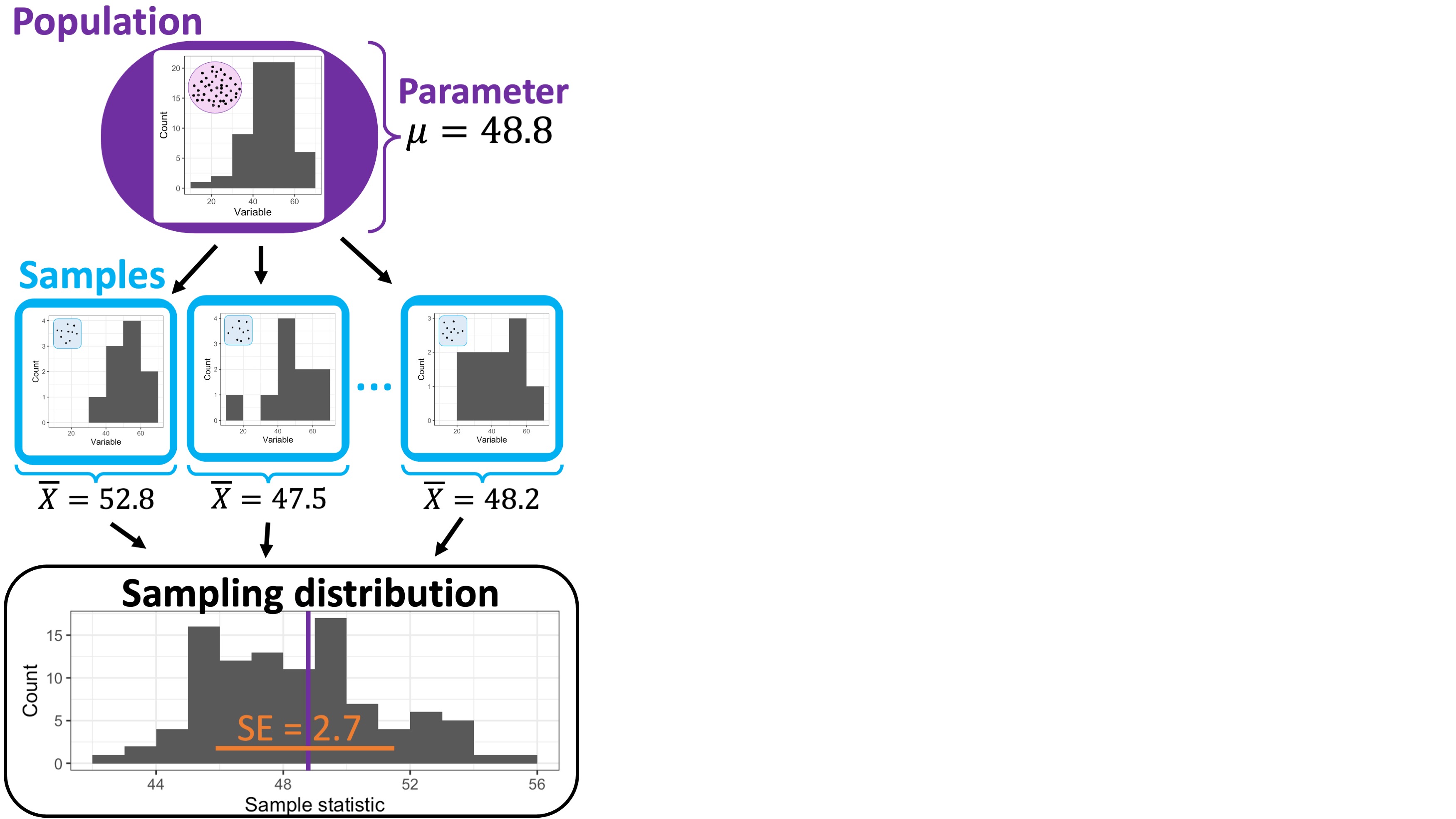
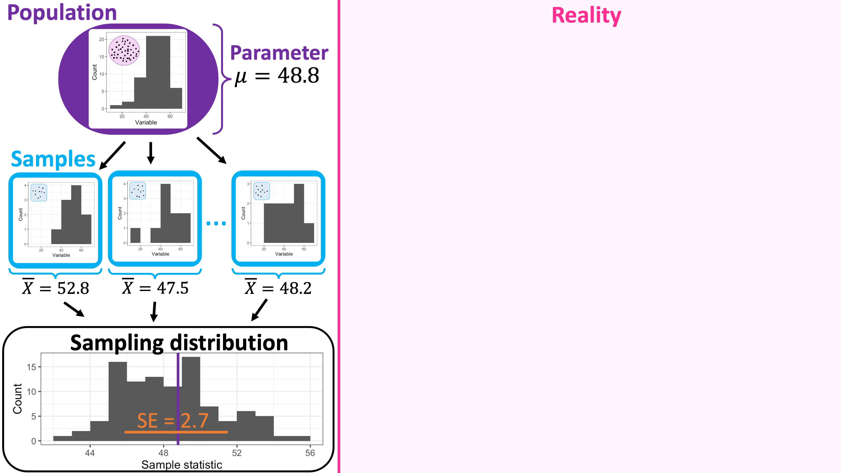
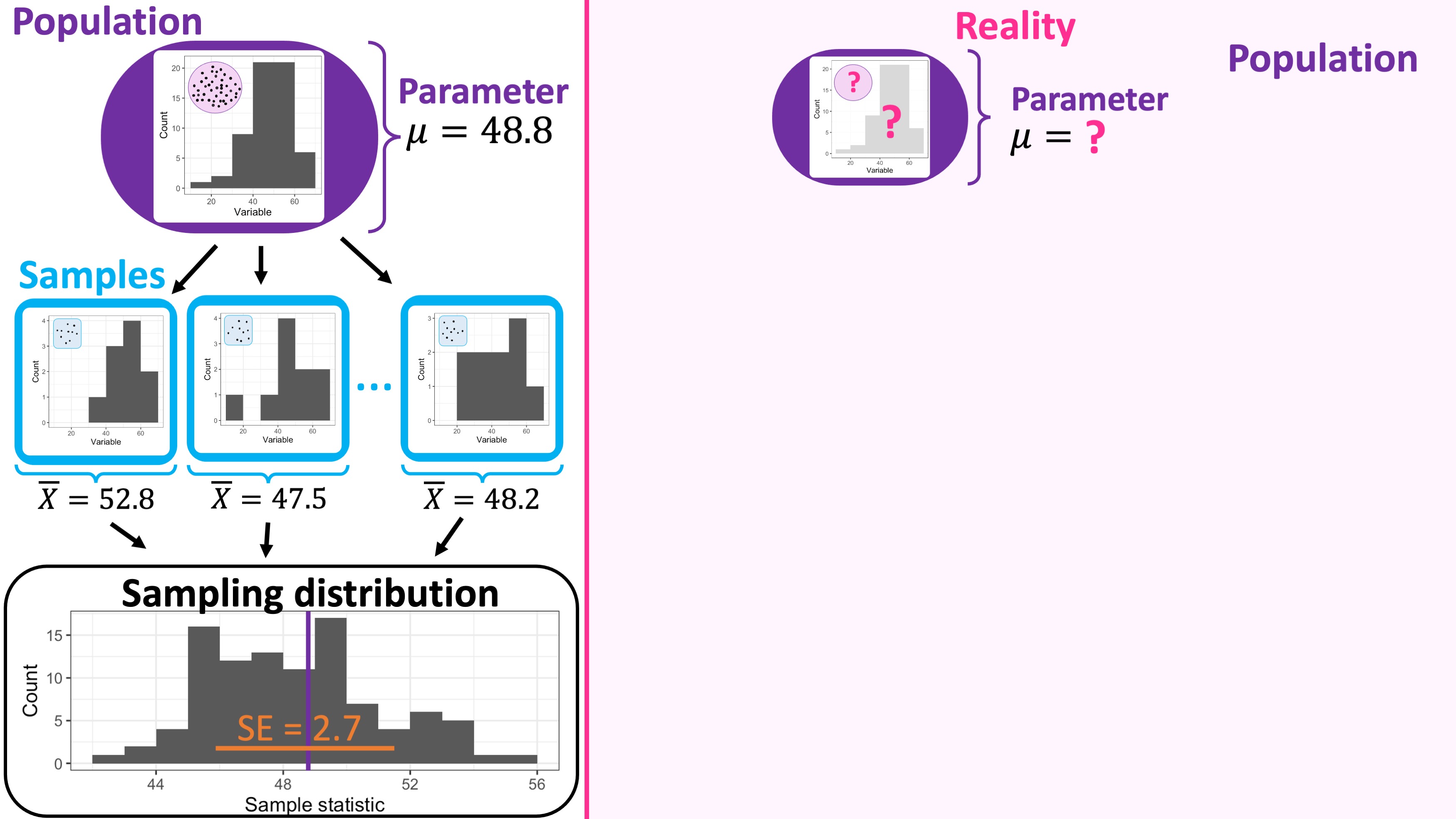
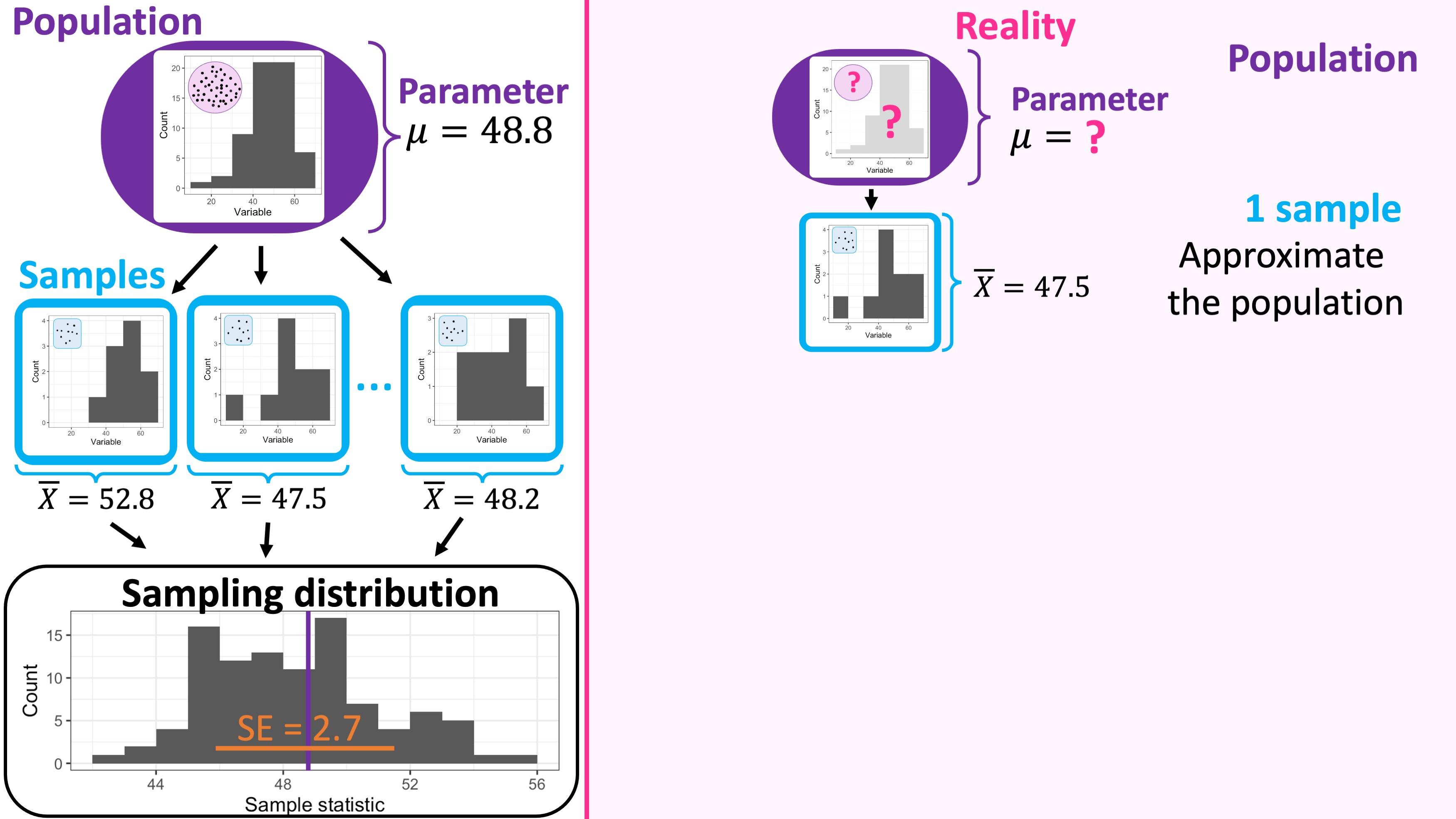
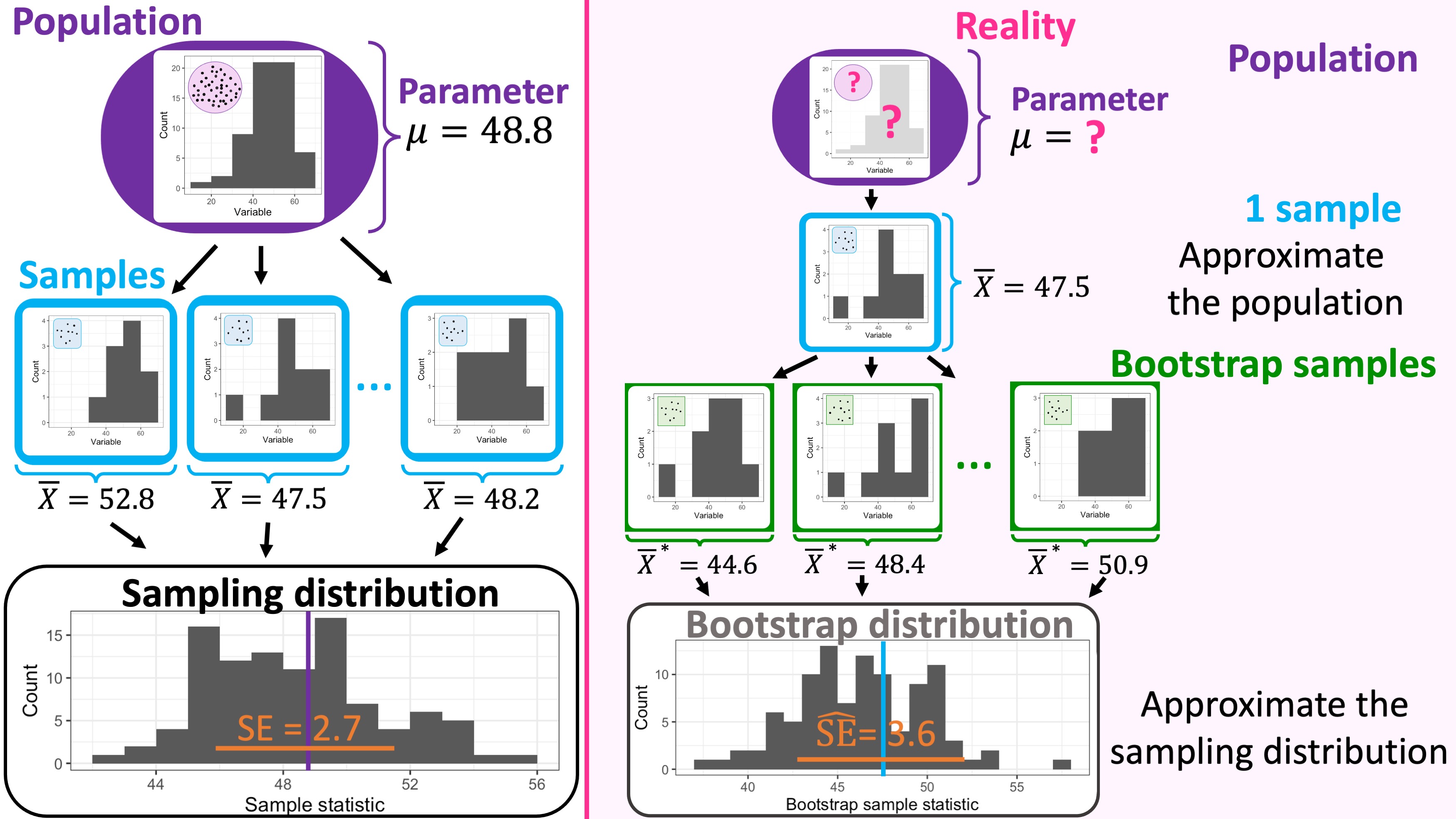
Estimating the sampling distribution via Bootstrapping (recap)

Sampling distribution of means is the distribution of the means of all the possible random samples of size \(n\) that could be selected from a population

Estimating the sampling distribution via Bootstrapping (recap)

Estimating the sampling distribution via Bootstrapping (recap)

Estimating the sampling distribution via Bootstrapping (recap)

Estimating the sampling distribution via Bootstrapping (recap)

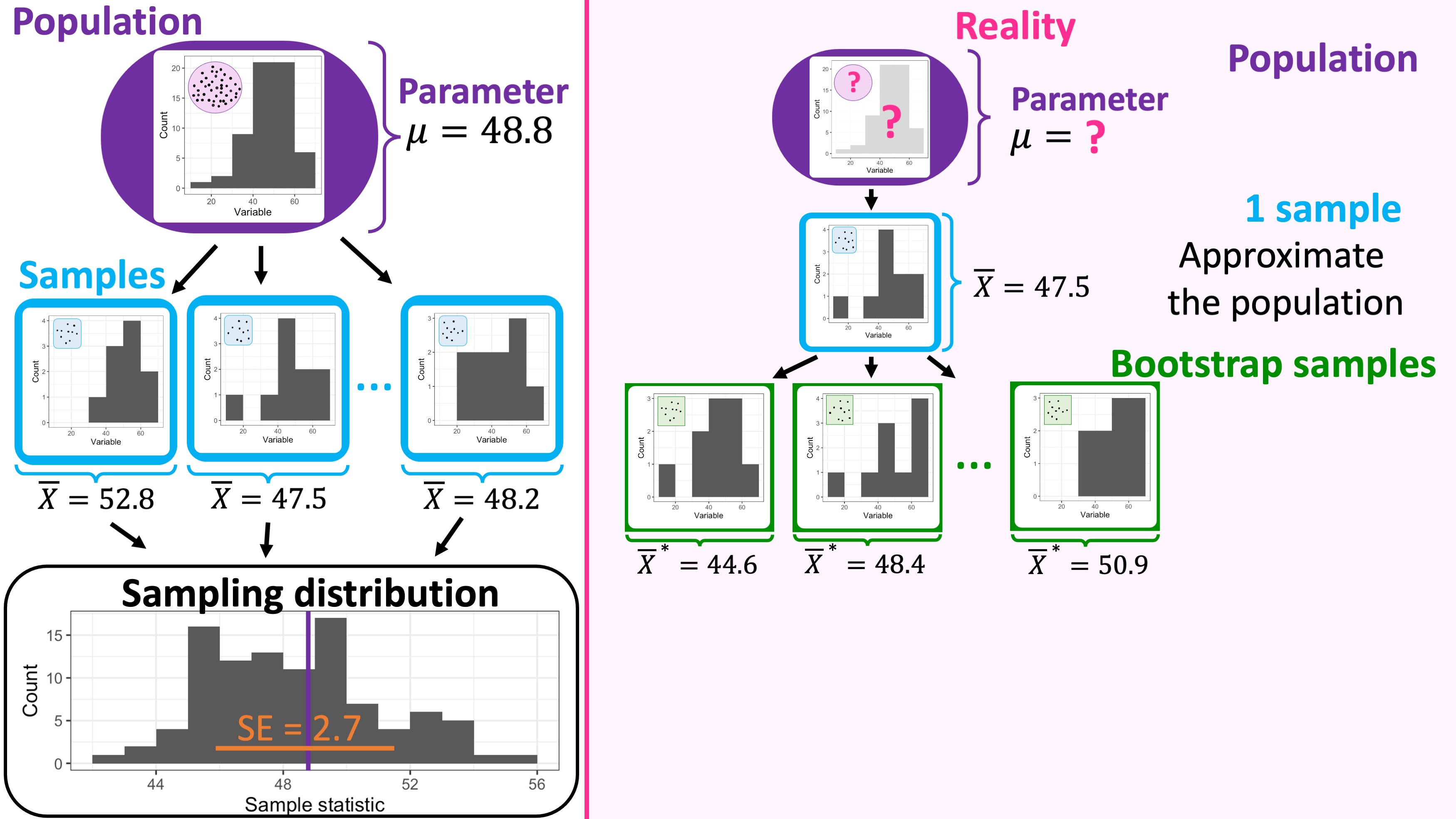
Estimating the sampling distribution via Bootstrapping (recap)

Why look beyond bootstrapping?

• In the previous module, we learned bootstrapping: a simulation-based approach to estimate the sampling distribution.

• While bootstrapping is extremely flexible, it has practical limitations:

  • It requires having the raw sample data.
  • It is computationally expensive for large datasets.
  • It is very unstable with small samples.

• But can we estimate the sampling distribution without running thousands of computer simulations?

• Today, we will explore a mathematical alternative.
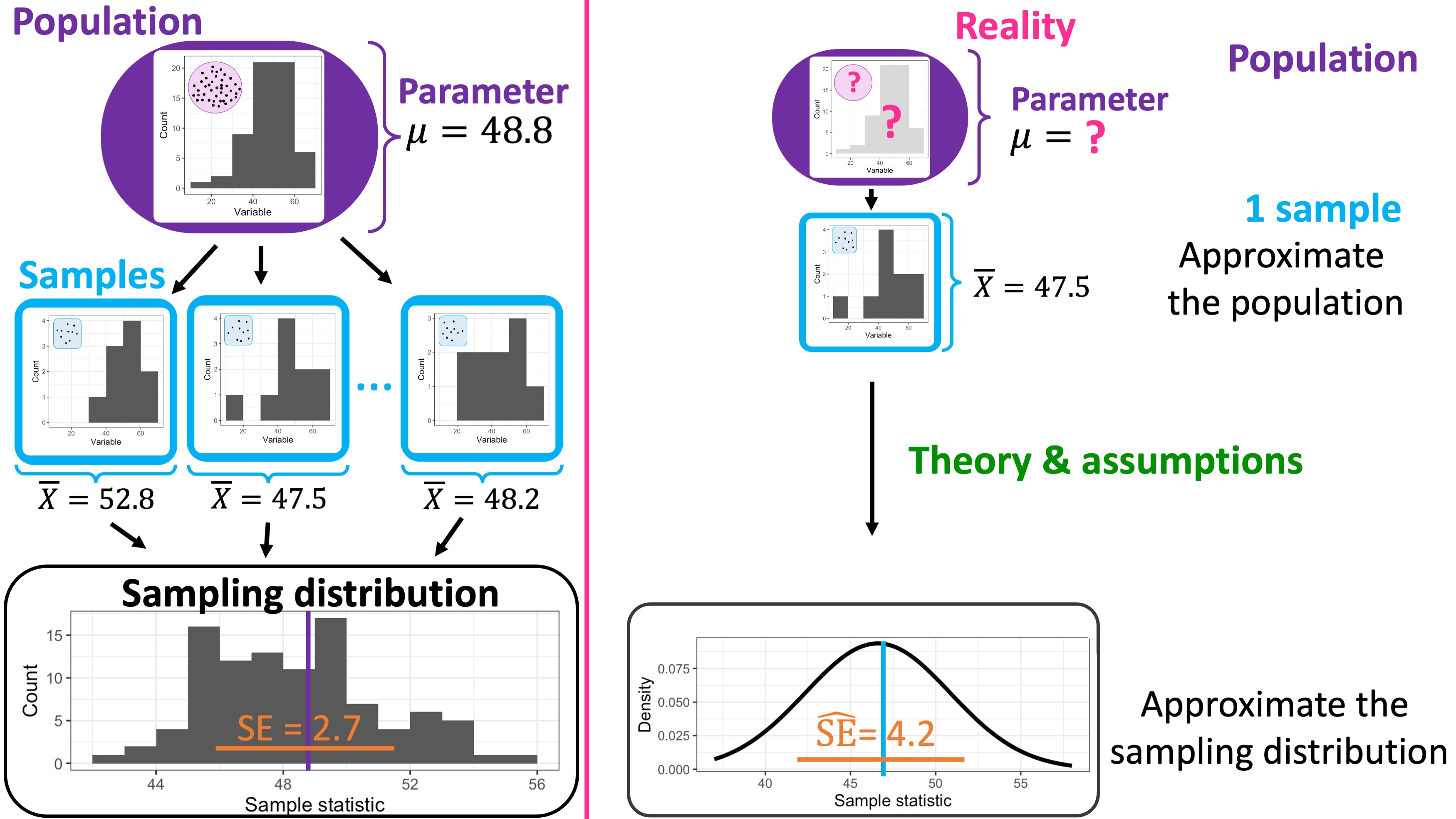
  • Instead of resampling our data, we will use probability theory to construct the sampling distribution directly.

• To do this, we need to understand three core pillars:
  • The Normal distribution
  • The Central Limit Theorem (CLT)
  • The Law of Large Numbers (LLN)

Estimating the sampling distribution via CLT

• Used for decades
• Relies on probability models and assumptions to construct the sampling distribution
• Contrast to the bootstrapping approach we’ve learned so far, which relies on computer simulations to construct the sampling distribution

Probability Distributions

Describing data with distributions

• Many different (and unrelated) measurements share common patterns;
• For example, if you collect data on:
  • the birthweights of newborns;
  • the wing lengths of houseflies; or
  • the resting heart rates of adults;
  you will find that the data tends to follow a common pattern: a symmetric, bell-shaped histogram;
• Similarly,
  • the number of Prussian soldiers killed by horse kicks in the 19th century
  • the number of goals scored in a soccer match
  • the number of typos per page in a book
  • the number of calls received by a call center
  might also follow a common pattern (a different one, which we won’t cover in this course).

• If we can find a mathematical model that describes the data well, we can:

  • Use it to answer questions about the data:

    • What is the proportion of newborns with weight between \(2.5\) kg and \(5\) kg?
    • What is the proportion of adults with a pulse rate above \(100\) beats per minute?
    • What is the birthweight threshold below which \(95\%\) of newborns fall?

  • Study properties of the distributions that will apply to other unrelated studies where the data have similar characteristics.

  • Summarize the data with just a few numbers (e.g., mean and standard deviation), while retaining the essential information (in the form of a probability distribution);

  • Smooth out random noise from our data (especially in small samples);

Do the data follow a common pattern?

The Normal Distribution

The Normal (Gaussian) Distribution

• It is arguably the most important statistical distribution, and it is used to model many natural phenomena.
  • It is also central in the context of sampling distributions, because of the Central Limit Theorem (CLT).

• The Normal distribution is characterized by two parameters:
  • the mean \(\mu\);
  • the standard deviation \(\sigma\).

Normal Model

Scroll down

viewof mu = {

  let input = Inputs.range([-5, 5], {value: 0, step: 0.1, label: "Mean"});
  
  d3.select(input)
  .select('input[name="number"]')
  .style("width", "75px");

  d3.select(input)
   .select('input[name="range"]')
   .style("width", "230px");

  return input;
}

viewof sigma = {
  let input = Inputs.range([0.3, 3], {value: 1, step: 0.1, label: "Standard Deviation"})
 
 d3.select(input)
   .select('input[name="number"]')
   .style("width", "50px");
  
  d3.select(input)
   .select('input[name="range"]')
   .style("width", "150px");
  
  return input;
}

range = (lower, upper, step) => {
  var size = (upper-lower)/step;
  
  return Array(size).fill().map((value, index) => {
    return lower + step * index
  });
};


normal_pdf = (x, mu, sigma) => {
  return x.map(value => {
    return Math.exp(-0.5 * ( (value - mu) **2 ) / (sigma**2))/(Math.sqrt(2 * Math.PI * sigma ** 2 ))
  });
};

garbage_variable = {


  d3.select("#normal-density")
    .selectAll("*")
    .remove()

  var margin = {top: 40, right: 30, bottom: 50, left: 100},
      width = 530 - margin.left - margin.right,
      height = 400 - margin.top - margin.bottom;

  // append the svg object to the body of the page
  var svg = d3.select("#normal-density")
    .append("svg")
      .attr("width", width + margin.left + margin.right)
      .attr("height", height + margin.top + margin.bottom)
    .append("g")
      .attr("transform",
            "translate(" + margin.left + "," + margin.top + ")");
  
  const data_x =  range(-10, 10, 0.01);
  const data_y_std = normal_pdf(range(-10, 10, 0.01), 0, 1);
  const data_y = normal_pdf(range(-10, 10, 0.01), mu, sigma);
  const data = data_x.map((value, index) => {
    return {'x': value, 'y_std': data_y_std[index], 'y': data_y[index]};
    });

    // Now I can use this dataset:
    // Add X axis --> it is a date format
    var x = d3.scaleLinear()
      .domain([d3.min(data, function(d) { return +d.x; }), d3.max(data, function(d) { return +d.x; })])
      .range([ 0, width ]);
    svg.append("g")
      .attr("transform", "translate(0," + height + ")")
      .call(d3.axisBottom(x));

    // Add Y axis
    var y = d3.scaleLinear()
      .domain([0, d3.max(data, function(d) { return +Math.max(d.y, d.y_std); })])
      .range([ height, 0 ]);
    svg.append("g")
      .call(d3.axisLeft(y));

    // Add the line
    svg.append("path")
      .datum(data)
      .attr("fill", "none")
      .attr("stroke", "steelblue")
      .attr("stroke-width", 1.5)
      .attr("d", d3.line()
        .x(function(d) { return x(d.x) })
        .y(function(d) { return y(d.y_std) })
        );
    
    svg.append("path")
    .datum(data)
    .attr("fill", "none")
    .attr("stroke", "red")
    .attr("stroke-width", 1.5)
    .attr("d", d3.line()
      .x(function(d) { return x(d.x) })
      .y(function(d) { return y(d.y) })
      );

  svg.selectAll('text')    
     .style('font-size', '14px');

  svg.append("text")
      .attr("class", "y label")
      .attr("text-anchor", "middle")
      .attr("y", x(-14))
      .attr("x", -y(0)/2)
      .attr("dy", ".75em")
      .attr("transform", "rotate(-90)")
      .style('font-size', '24px')
      .text("Density");

  svg.append("text")
    .attr("class", "x label")
    .attr("text-anchor", "middle")
    .attr("x", x(0))
    .attr("y", height + 45)
    .style('font-size', '24px')
    .text("x");

   svg.append("text")
        .attr("x", width / 2)
        .attr("y", 0)
        .attr("text-anchor", "middle")
        .text("Normal Curve")
        .attr("dy", "-15px")
        .style('font-size', '32px')
        .attr("class", "plot-title");

  svg.append("rect")
    .attr("x", x(6))
    .attr("y", 40)
    .attr("width", 20)
    .attr("height", 2)
    .style("fill", "steelblue")
  svg.append("text")
    .attr("x", x(7.5))
    .attr("y", 45)
    .text("N(0, 1)")
    .style("font-size", "15px")
    .attr("alignment-baseline","middle")

  svg.append("rect")
    .attr("x", x(6))
    .attr("y", 60)
    .attr("width", 20)
    .attr("height", 2)
    .style("fill", "red")
  svg.append("text")
    .attr("x", x(7.5))
    .attr("y", 65)
    .text('N(' + mu + ', '+ (sigma**2).toPrecision(2) +')')
    .style("font-size", "15px")
    .attr("alignment-baseline","middle")


};

• Properties:

  • Bell-shaped and unimodal;

  • Fully specified by two parameters, \(\mu\) and \(\sigma\):

    • \(\mu\) determines the location;

    • \(\sigma\) determines the spread;

  • Symmetric about the mean \(\mu\);

Areas under the Normal Model

• The area under the Normal model tells us the probability that the corresponding variable is in a specified region.

• We need to use computers to obtain the area under the Normal model (there’s no closed-form solution).

• But there’s a rule that can help us do a quick check of our calculations.

The 68-95-99.7% Rule

Scroll down

No matter the values of \(\mu\) and \(\sigma\), we have the following rule

Interval	% of data within the interval
within \(1\sigma\) of \(\mu\)	about \(68\%\)
within \(2\sigma\) of \(\mu\)	about \(95\%\)
within \(3\sigma\) of \(\mu\)	about \(99.7\%\)

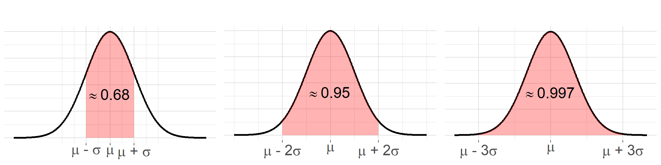
• This is a useful approximation for a sanity check.
  • For actual solutions, we use R.

R’s pnorm and qnorm functions

Scroll down

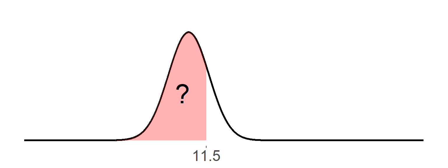
Probability:

• To obtain the area under the curve, we use the pnorm function.

• For example, suppose we have a \(N( \mu = 10, \sigma^2 = 3)\) and want the area below 11.5:

• We can use the following code

pnorm( 11.5, mean = 10,  sd = sqrt(3))  

[1] 0.8067619

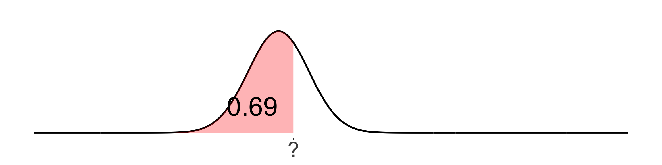
Quantile:

• To obtain the quantile of a Normal, we use the qnorm function.

• For example, suppose we have a \(N( \mu = 10, \sigma^2 = 3)\) and want the 0.69-quantile:

• We can use the following code

qnorm( 0.69, mean = 10,  sd = sqrt(3))

[1] 10.85884

Standard Normal

• The Normal distribution with \(\mu=0\) and \(\sigma^2=1\) is called the Standard Normal distribution, i.e., \(N(0, 1)\).

• We can always convert a Normal random variable to a Standard Normal by subtracting the mean and dividing by the standard deviation.

• For example, imagine you have a variable height, and you want to convert it to a Standard Normal variable. You can use the following code:

standardized_height <- (height - mean(height)) / sd(height)

Diagnostics

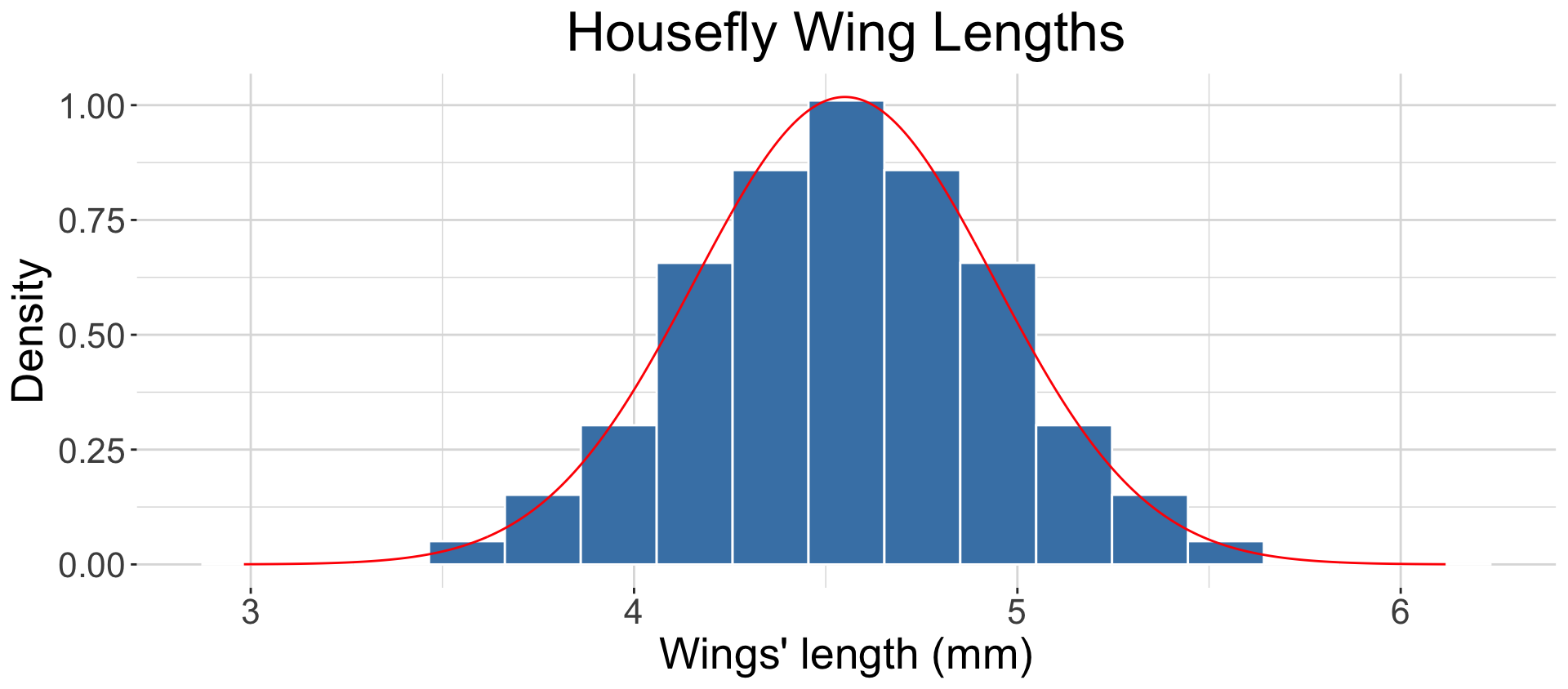
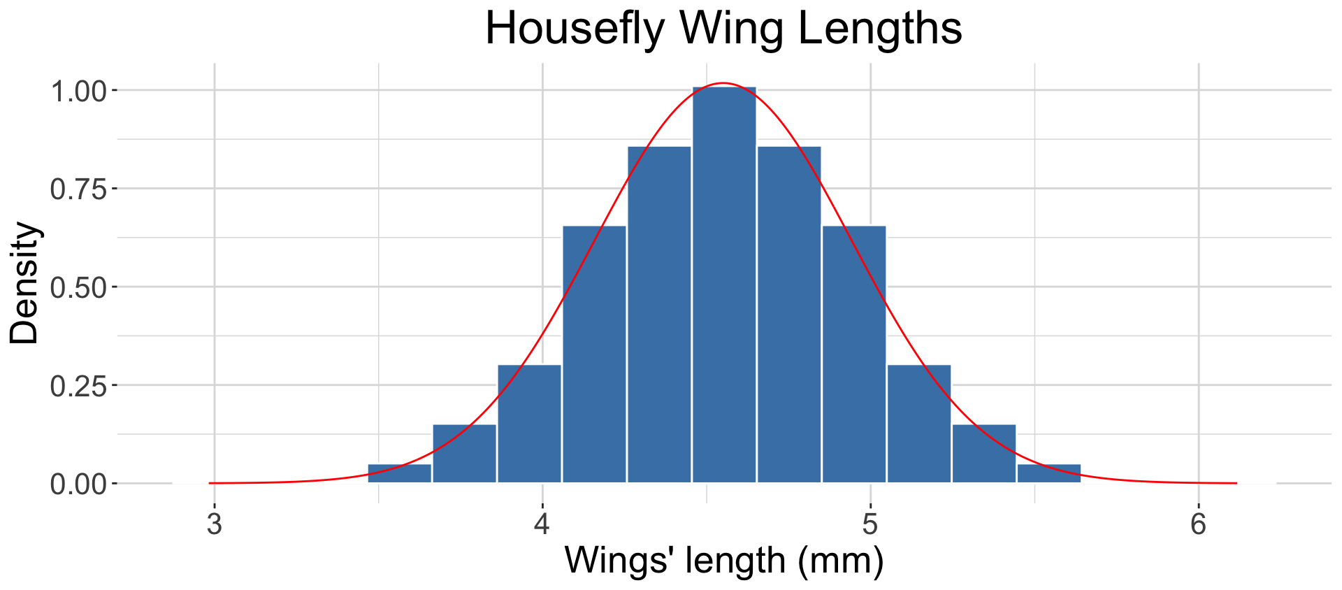
• There are multiple ways to check the adequacy of the Normal model. A simple (and subjective) way is to check if the relative frequency histogram looks like a Normal curve.

Example 1: Housefly Wing Lengths

• Sokal and Hunter (1955) studied the wing lengths of houseflies.

Example 2: Birthweight

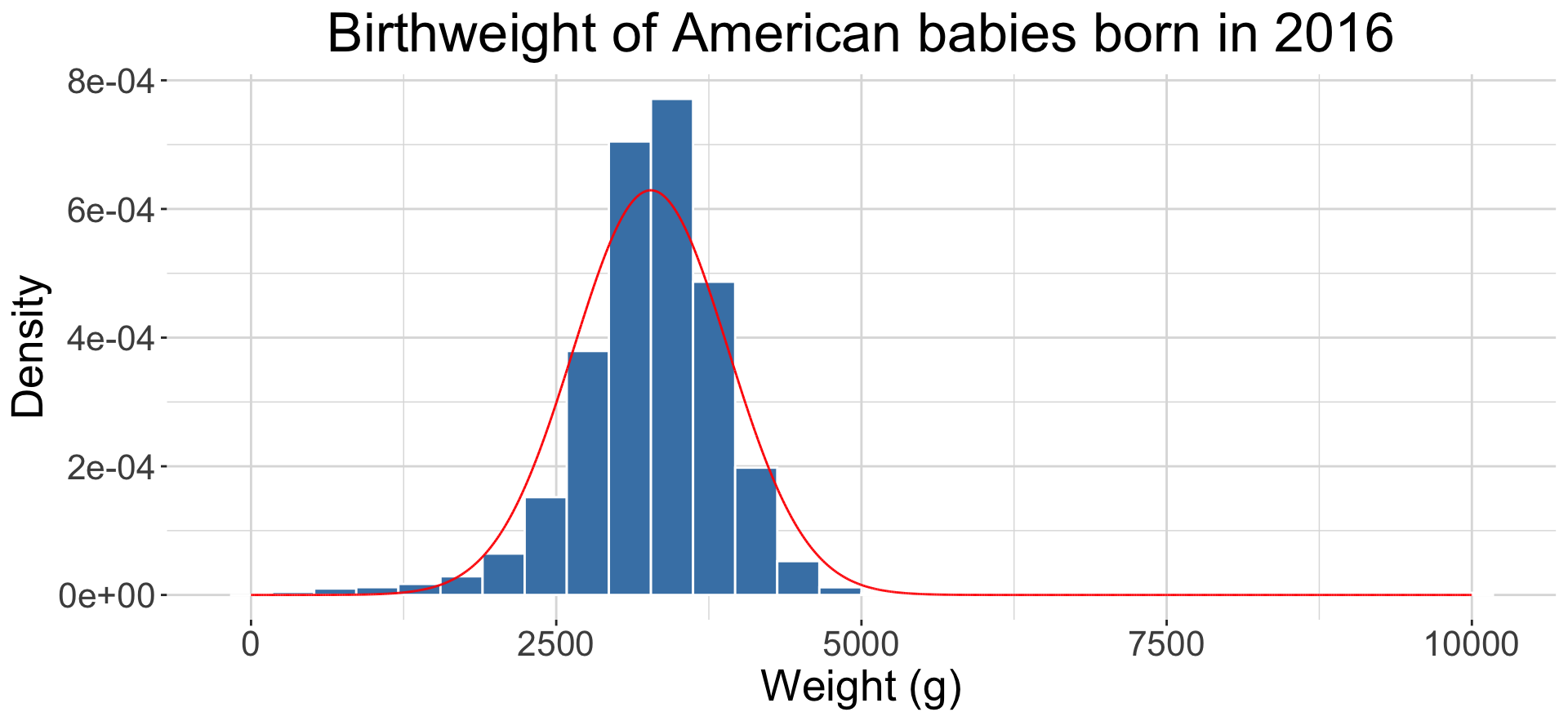
In this case, we have a heavier left tail, which might compromise the Normal approximation.

The Central Limit Theorem (CLT)

Central Limit Theorem (CLT)

• The Central Limit Theorem helps us to approximate the sampling distribution of certain statistics.

• In loose words, the CLT states that no matter what the population is, the sampling distribution of certain statistics, such as the sample mean and the sample proportion, approximates the Normal distribution for large sample sizes.

CLT for the Sample Mean

Scroll down

• For large sample sizes, the sampling distribution of the sample mean is approximately: \[\bar{X} \sim N\left(\mu, \frac{\sigma^2}{n}\right)\] regardless of the population distribution.

• The mean of the sampling distribution is the population mean \(\mu\).

• The standard error is: \[SE(\bar{X}) = \frac{\sigma}{\sqrt{n}}\] where \(\sigma\) is the population standard deviation.

Exact Results for Normal Populations

If the population distribution is Normal, then the sampling distribution \(\bar{X} \sim N\left(\mu, \frac{\sigma^2}{n}\right)\) is an exact result for any sample size. In this scenario, we do not need the CLT.

CLT for the sample proportion

Scroll down

• For large sample sizes, the sampling distribution of \(\hat{p}\) is approximately: \[{\hat{p}} \sim N\left(p, \frac{p(1-p)}{n}\right)\]

• The mean of the sampling distribution is the population proportion \(p\).

• The standard error is: \[SE(\hat{p}) = \sqrt{\frac{p(1-p)}{n}}\]

Recall: The sampling distribution of proportions is the distribution of the sample proportions of all possible random samples of size \(n\) that can be obtained from a population.

The larger the sample size n, the better the normal approximation.

Sample size effect on the sampling distribution (Normal)

Sample size effect on the sampling distribution (Not-Normal)

Assumptions & conditions

• Sample is randomly drawn from the population
• Sample values are independent
  • Generally, if your sample size is greater than 10% of the population size, the violation of independence becomes too large to ignore.
• Sample size must be large enough.
  • For means:
    • There is no universal guideline for how large \(n\) should be.
    • Usually, a sample size greater than \(30\) is large enough to get a reasonable approximation — though this is not guaranteed.
  • For proportions:
    • We check whether \(n \times p \ge 10\) and \(n \times (1-p) \ge 10\).

Standard Error (SE)

• The standard error is the standard deviation of a point estimator.

• Mean — The standard error of the sample mean is: \[SE(\bar{X}) = \frac{\sigma}{\sqrt{n}}\] where \(\sigma\) is the population standard deviation.

• Proportion — The standard error of the sample proportion is: \[SE(\hat{p}) = \sqrt{\frac{p(1-p)}{n}}\] where \(p\) is the population proportion.

• In practice, we rarely know the population parameters, so we substitute them with sample estimates.

• Mean — We estimate the standard error as: \[\widehat{SE}(\bar{X}) = \frac{s}{\sqrt{n}}\] where \(s\) is the sample standard deviation.

• Proportion — We estimate the standard error as: \[\widehat{SE}(\hat{p}) = \sqrt{\frac{\hat{p}(1-\hat{p})}{n}}\] where \(\hat{p}\) is the sample proportion.

The Law of Large Numbers (LLN)

The Law of Large Numbers (LLN)

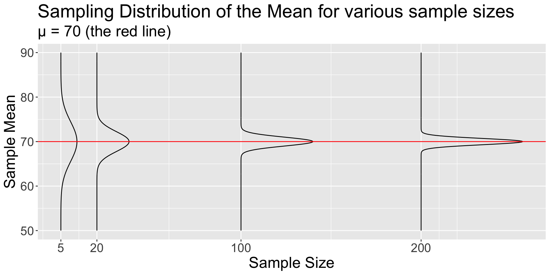
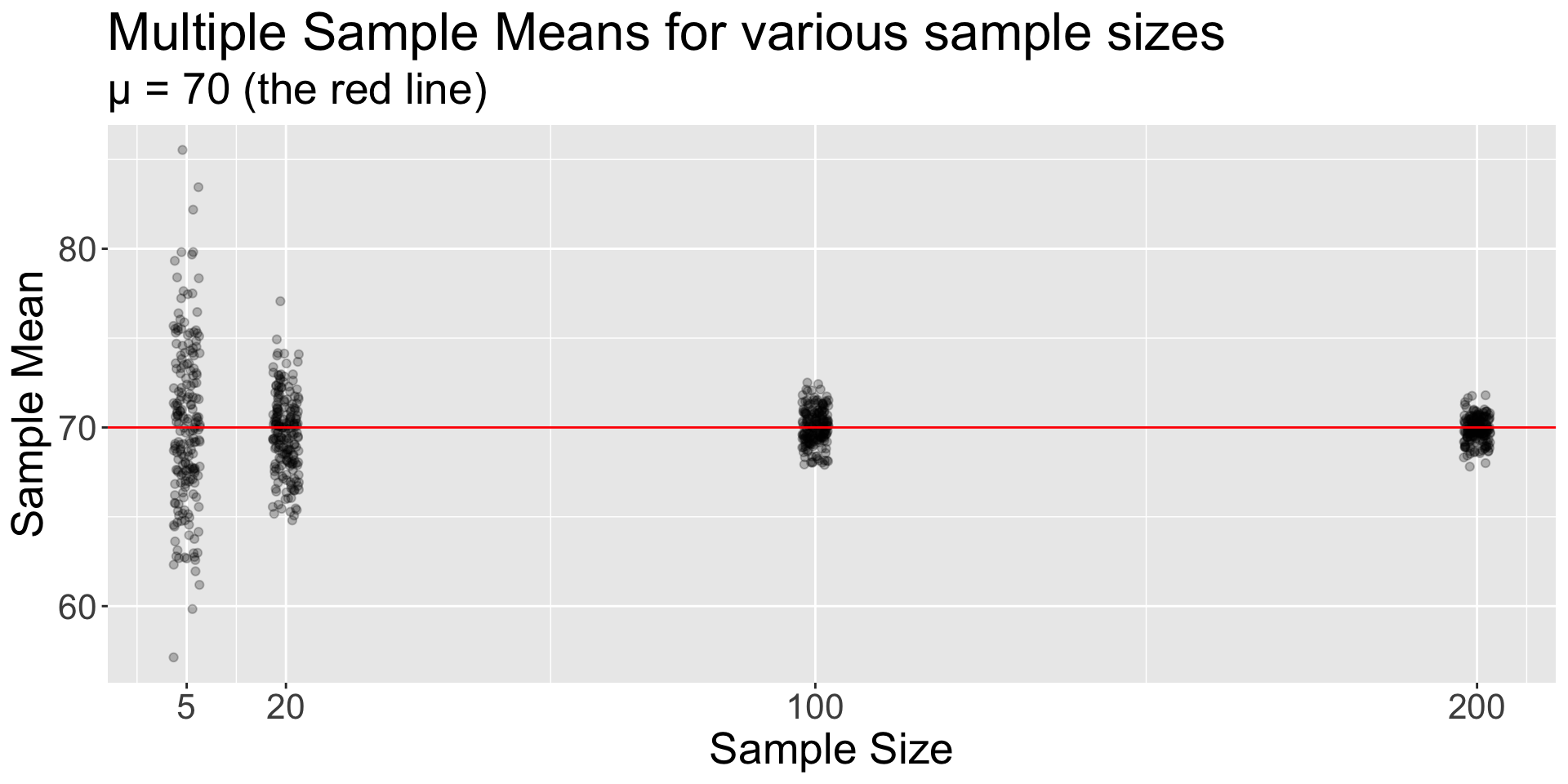
• The Law of Large Numbers states that as the sample size increases, the sample mean converges to the population mean.

• In other words, as we collect more and more observations, the sample mean eventually settles arbitrarily close to the population mean.

The Law of Large Numbers

• The law of large numbers is actually intuitive given what we have seen so far.

The Law of Large Numbers

Bootstrapping or the CLT?

• Both approaches estimate the same thing: the sampling distribution of an estimator.

• Advantages and disadvantages of Bootstrapping:

  • Highly unstable for small samples;
  • Can be used for virtually many estimators, even those without a usable asymptotic result;
    • Caution: may not perform well for extreme quantiles or tail probabilities.
  • Computationally intensive, especially for large samples;

• Advantages and disadvantages of CLT:

  • The Normal approximation may be poor for small samples;
    • However, the results tend to be superior to the bootstrap for small samples (say \(n\leq 30\));
  • Only works for certain estimators (e.g., sample mean, sample proportion);
  • Computationally cheap, can be computed almost instantly, even for large samples;

To Take Home

Take home: CLT

• The CLT only works for certain statistics (e.g., the sample mean and the sample proportion).

• As the sample size increases, the sampling distribution of the sample mean and the sample proportion becomes narrower, more symmetric, and more bell-shaped.

Take home: Std. Errors

• The standard errors:
  • \(SE(\bar{X}) = \frac{\sigma}{\sqrt{n}}\)
  • \(SE(\hat{p}) = \sqrt{\frac{p(1-p)}{n}}\)
• These formulae do not depend on the CLT. They are valid for all sample sizes.

Take home: LLN

• The Law of Large Numbers guarantees that the sample mean converges to the population mean as the sample size increases.

• The CLT describes the shape of the sampling distribution; the LLN describes where it concentrates.

Today’s worksheet

• Investigate the law of large numbers and the central limit theorem
• See that the sampling distributions for the sample mean/proportion can be well approximated by the Normal distribution when the sample size is large, regardless of the distribution of the population

References

Sokal, Robert R., and Preston E. Hunter. 1955. “A Morphometric Analysis of Ddt-Resistant and Non-Resistant House Fly Strains1, 2.” Annals of the Entomological Society of America 48 (6): 499–507. https://doi.org/10.1093/aesa/48.6.499.